
Loading...
Loading...
Loading...
Loading...
Loading...
Loading...
Loading...
Loading...
Loading...
Loading...
Loading...
Loading...
Loading...
Loading...
Loading...
Loading...
Loading...
Loading...
Loading...
Loading...
Loading...
Loading...
Loading...
Loading...
Loading...
Loading...
Loading...
Loading...
Loading...
Loading...
Loading...
Loading...
Loading...
Loading...
Loading...
Loading...
Loading...
Loading...
Loading...
Loading...
Loading...
Loading...
Loading...
Loading...
Loading...
Loading...
The chapter provides instructions and examples of using computing skills for health data and technology research.
Instructions for installing Julia on macOS and Windows operating systems can be found here.
Package managers such as Homebrew (macOS and Linux) and Chocolatey (Windows) can be used to facilitate installation.
For most users, it is recommended to download the current stable release from https://julialang.org/downloads/.
Some developers might wish to use a different version, or to switch between versions. For this, the Juliaup version manager can be useful.
Julia is also available for use in Brown's Computing Environments:
Oscar (for high-performance computing)
Stronghold (for secure computing)
Julia is an open source dynamic programming language for high-level, high-performance numerical computing [1]. Julia provides ease and expressiveness (similar to R, MATLAB, and Python), but also supports general programming [2].
Development of Julia began in 2009, and the first version was released in February 2012. The current version of Julia is 1.11 (as of November 2024).
Learn X in Y Minutes: X=Julia
Programming languages are written using text editor applications. These applications allow users to create and edit free text, which can then be run as programs. Text editors differ in complexity, some including extra functionality for easier, more efficient programming. Text editors with auto-complete suggest common functions or existing variables as the programmer begins to type, which the programmer can then select without needing to finish typing. Some text editors offer options to run individual lines of code or entire programs while editing files.
Available for Mac, Windows, and Linux operating systems
Includes support for debugging, syntax highlighting, auto-complete, and additional user-friendly functionality
Web application text editor, no download necessary
Includes options for interactive output (HTML, images, videos, LaTeX, and custom MIME types), support for big data tools, such as Apache Spark, and options for sharing notebooks with others
Run individual lines of code or entire programs at once
Highly configurable
Included in most UNIX operating systems (e.g., Linux, or MacOS), no download necessary
Write files from the Terminal
Highly configurable
Included in most UNIX operating systems (e.g., Linux, or MacOS), no download necessary, also available for Windows
Wide range of built-in features for text editing, such as syntax highlighting, automatic indentation, and search and replace
Included in most UNIX operating systems (e.g., Linux, or MacOS), no download necessary
Most of the editing commands are displayed at the bottom of the editing screen for easy reference
List of exercises found across the different Julia pages.
Use Julia in Brown Oscar Computing Environment - Forthcoming!
Use Julia in Brown Stronghold Computing Environment - Forthcoming!
Create a Health Calculator Using Julia - Forthcoming!
Create a Pediatric Dosage Calculator Using Julia
Create a BMI Calculator Using Julia
Analyze Health Datasets Using Unix Commands - Forthcoming!
Analyze MIMIC-IV Demo Files Using Unix Commands
Analyze SyntheticRI Demo Files Using Unix
Analyze Health Datasets Using Julia - Forthcoming!
Analyze MIMIC-IV Demo Files Using Julia
Analyze SyntheticRI Demo Files Using Julia
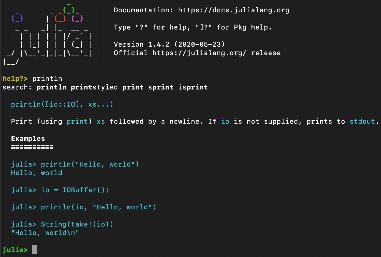
Julia comes with a full-featured interactive command-line REPL (read-eval-print loop) built into the
juliaexecutable. In addition to allowing quick and easy evaluation of Julia statements, it has a searchable history, tab-completion, many helpful keybindings, and dedicated help?and shell modes;. [1]
This page provides examples of using REPL on the command line.
Type julia in terminal to launch REPL
Type "?" to enter help pages within REPL
Type a function from Julia to read help pages (ex: println)
Julia Contributors. (n.d.). REPL - Standard Library - Julia Language. Retrieved May 1, 2024, from https://docs.julialang.org/en/v1/stdlib/REPL/
Julia Documentation: The Julia REPL
Julia Cheat Sheet (see REPL)
GitHub is a code hosting platform that allows developers to create, store, manage, and share their code. It uses Git software, providing the distributed version control of Git plus access control, bug tracking, software feature requests, task management, continuous integration, and wikis for every project. Refer to for additional GitHub documentation and tutorials.
Like other cloud platforms (e.g., Google Docs), GitHub allows users to work on projects together. Please note, code changes must be manually saved. GitHub does not automatically save your work. To save changes, open the Terminal application, navigate to the cloned repository, and run the following commands, replacing "INSERT PROGRESS NOTE" with brief description of changes.
git add -A : adds all your code changes to the GitHub repository
git commit -m"INSERT PROGRESS NOTE" : adds a note to the commit which you and your team can reference later. This note should be brief and informative, describing the purpose of your code changes.
git push : saves your code changes to the GitHub repository.
If multiple users are pushing code changes to your GitHub repository, make sure to retrieve or "pull" these edits before you begin making code changes. To do so, open the Terminal application, navigate to the cloned repository, and run the following command. If you have made any code changes, you will need to save them first for the pull to work.
When your are making code changes, you should git pull before making any edits. This will keep your team from encountering "merge conflicts", which can become difficult to troubleshoot. To mitigate merge conflicts, make sure to communicate with your team. Inform your team whenever you push new code changes so that everyone is always working one the most updated version of the code.
Merge conflicts happen when you attempt to merge code branches that have competing commits. They are often caused by users making code changes without pulling first. To resolve a merge conflict, work through the following steps:
Identify the location of the merge conflict.
Manually edit the conflicted file from a single machine, selecting the changes you want to keep in the final merge.
Push the selected changes to GitHub.
All team members should pull the corrected changes from GitHub before continuing to make code changes.
All major operating systems organize files into hierarchical directories. Understanding these file directory structures is vital when interacting with data files using Unix commands or a programming language.
This page describes file directory structures generally as well as some of the differences between file directory structures within different operating systems.
Directories allow users to group files into an organized structure. They are typically visualized like root systems of trees, the highest level of which is called the "root directory". Subdirectories branch down from the root directory, containing files as well as additional subdirectories.
Directories and files are typically described using the path used to reach them through the directory structure, starting with the root directory. In Linux and Mac operating systems, the root directory is indicated as "/" (In Windows OS, the root directory is indicated as "\"). An additional "/" (or "\" for Windows OS) is placed between each object in the path.
For example, looking at Figure 1, File_B1a2 could be described with:
/Directory_B/Directory_B1/Directory_B1a/File_B1a2
All major operating systems also provide users with a graphical user interface, or GUI (often pronounced "gooey"), which allows interaction with software and files through visual icons. If you are not already familiar with accessing files and directories through the command line, you are likely familiar with using a GUI file system. While not the recommended method for interacting with files while programming, the GUI file system can be a useful tool for visualizing a directory structure.
Figure 2 displays the GUI file system for a computer running MacOS. Though the GUI directory structure is visualized horizontally, the "root system" is still clearly visible. Using its complete path, the file "medication_data" should be described as:
/Users/<username>/Documents/project_a/data_files/medication_data
git add -A
git commit -"INSERT PROGRESS NOTE"
git pushgit pullR is one of the many languages used by the data science community to perform data manipulation, statistical modeling and machine learning. R was designed by statisticians for statistical computing.
In computer programming, a package is a collection of modules or programs that are often published as tools for a range of common use cases, such as text processing and doing math. Programmers can install these packages and take advantage of their functionality within their own code.
This page provides instructions for installing, using, and troubleshooting packages in Julia.
Start Julia REPL by typing the following in Terminal or PowerShell (Note: do not need to type $ - this is to indicate the shell prompt)
$ juliaGo into REPL mode for Pkg, Julia’s built in package manager, by pressing ]
$ julia ]$ (@v1.4) pkg>Update package repository in Pkg REPL
$ (@v1.4) pkg> updateAdd packages in Pkg REPL
$ (@v1.4) pkg> add CSV$ (@v1.4) pkg> add DataFramesCheck installation
(@v1.4) pkg> status
            Status `~/.julia/environments/v1.0/Project.toml`
                [336ed68f] CSV v0.4.3
                [a93c6f00] DataFrames v0.17.1
                ...
Get back to the Julia REPL and exit by pressing backspace or ^C.
(@v1.4) pkg>

julia>
To see REPL history
$ more ~/.julia/logs/repl_history.jljulia> using CSV
julia> using DataFrames
julia> exit()If you get an error like: ERROR: SystemError: opening file "C:\\Users\\User\\.julia\\registries\\General\\Registry.toml": No such file or directory
Delete C:\\Users\\User\\.julia\\registries where User is your computer’s username and try again
https://discourse.julialang.org/t/registry-toml-missing/24152
JuliaHealth and BioJulia organizations (focused on Julia packages for health and life sciences)
Julia Package: CSV.jl
Julia Package: DataFrames.jl
JuliaStats contains basic statistics functionality, which can be used as the foundation for statistics, machine learning, and data science needs. It is efficient, scalable, and reusable!
JuliaStats is not a single package, but rather a suite of packages. Specific packages can be downloaded depending on your needs.
To begin, import the package manager and initialize your desired package with the following code.
import Pkg
Pkg.add(*package name*)

using *package name*
For example, if you wanted to download the StatsBase package, use the following code.
import Pkg
Pkg.add("StatsBase")

using StatsBaseStatsBase.jl
Basic statistics, weights, sampling, counts, and summary statistics.
Distributions.jl
Probability distributions and related functions (PDF, CDF, sampling, etc).
StatsModel.jl
Statistical model formulas
GLM.jl
Generalized linear models (e.g., linear regression, logistic regression).
MixedModels.jl
Linear and generalized linear mixed-effects models.
HypothesisTest.jl
Statistical hypothesis tests (t-tests, chi-squared, ANOVA, etc).
MultivariateStats.jl
Multivariate analysis (PCA, factor analysis, ICA, etc).
Please refer to each package's documentation for a list of available functions and their usage.
# Using StatsBase
data = ..
mean_val = mean(data)
var_val = var(data)

# Using Distributions
pdf_val = pdf(Normal(0,1), 1)

# Using GLM
df = DataFrame(..)
model = lm(@formula(y ~ x), df)Get string length
nchar(string)
Combine two strings
str_c(string1, string2)
Sort values within a string
sort(string1, string2, string3)
#String length
nchar("codiac")

#Combine strings
str_c("patient ", c("a", "b", "c"))

#Sort values in a string
x <- c("carrot", "apple", "banana")
sort(x)#String length
6
#Combine strings
"patient a" "patient b" "patient c"
#Sort values in a string
"apple" "banana" "carrot"R for Data Science: String Functions
In computer programming, a package is a collection of modules or programs that are often published as tools for a range of common use cases, such as text processing and doing math. Programmers can install these packages and take advantage of their functionality within their own code.
This page provides instructions for installing, using, and troubleshooting packages in Python.
There is a two-step process for using an external package in Python. First, if it is your first time using the package, you must install the package. This only needs to be done once for the environment you are working in, even if you are using different documents or files. Then, you must load the package to your specific document. Let's look at an example using the NumPy package
To install a package, we use the pip command as follows:
pip install numpyAgain note that this only needs to be done once. After you have installed a package you do not need to do so again, you can simply load it
If we want to load an entire package (instead of just certain functions), we can use the import command as follows:
import numpy as npWe import the name of the package and name is as some shorthand name so that we do not need to type the whole package name every time we want to use a function from that package. In order to call a function from an imported package we can use the shorthand name followed by a dot followed by the name of the function. Here is an example:
# Creating an array
array1 = np.array([1, 2, 3, 4, 5])

# Getting the mean of the values in our array
mean = np.mean(array1)
Some packages will have many different parts, or modules, and we might not want to use all of these modules at once. Importing all of these modules when we don't need them can be an unnecessary waste of computing power, so instead we can only import the functions we need. Let's look at the scikit-learn package for example
We can install this package the same way as above, however we will not import the whole package at once. Instead, we will only import the functions we need from the modules we need. Here is an example of how we can import the train_test_split() function from the model_selection module of scikit-learn (or sklearn for short)
from sklearn.model_selection import train_test_splitIn computer programming, a package is a collection of modules or programs that are often published as tools for a range of common use cases, such as text processing and doing math. Programmers can install these packages and take advantage of their functionality within their own code.
This page includes instructions for installing packages in R and a description of some of R's most frequently used packages.
To install a package in R, you can either:
Use the install.packages("PackageName") function if you have the package downloaded locally on your machine
Or if you are using RStudio, you can use Tools > Install packages, enter in the package name and click Install
Once you install the package, you have to load it into your library using the libary(PackageName) function.
#Installing a package downloaded locally
install.packages("tidyverse")

#Once the package is installed, you have to load it
library(tidyverse)In R, tidyverse is one of the most popular packages, as it contains an assortment of packages used for data science, such as:
ggplot2, used to create graphics and data visualization
dplyr, contains functions used for data manipulation, like mutate() and filter()
tidyr, used for data organization and cleaning
tibble, an optimized dataframe visualizer
readxl, can be used to input Excel files in .xlsx format into R
R Documentation: Packages
Python comes with a full-featured interactive command-line REPL (read-eval-print loop) built into the
pythonexecutable. In addition to allowing quick and easy evaluation of Python statements, it has a searchable history, tab-completion, many helpful keybindings, and dedicated help?and shell modes;.
This page provides examples of using REPL on the command line
Type python in terminal to launch REPL
Type "help" to enter help pages within REPL
Type a function from Python to read help pages (ex:print)
Press q to quit
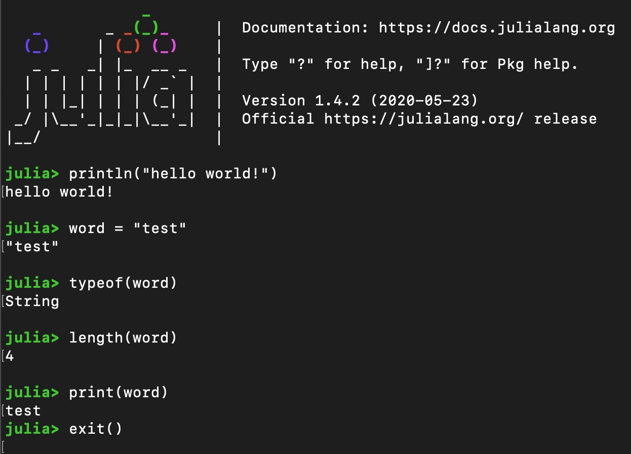
This is the typical first program for those new to a general purpose programming language like Julia. It can be used to test that the of Julia is working and also introduce Julia's basic syntax using the environment or running code written using a at the command line.
Input:
Output:
Here are variations of the "Hello, World!" programming using variables and different print statements.
Input:
Output:
In order to assign variables in Julia, you write the desired name for your variable, an = sign, and what the value of the variable should be.
Input:
Output:
We can write comments on our code, which do not run, to describe what certain lines of code or section of code do
These comments are just for the programmer, they will not appear anywhere in the output and just are there to explain what the code is doing or to provide helpful notes
To make a comment in Julia, you can use the “#” symbol and then type your comment
Sometimes you might want to write longer comments that span multiple lines – to do this you can surround these comments with #= above the start as well as =# below the end
Input:
Output:
Without using a print statement, Julia will only print out the most recent item that has an output. In order to print multiple things, we can use the print() or println() functions.
Input:
Output:
Use Julia in Brown Oscar Computing Environment - Forthcoming!
Use Julia in Brown Stronghold Computing Environment - Forthcoming!
Julia Documentation:
Julia Documentation:
Think Julia:
Think Julia:
ScikitLearn.jl lets you use many stats packages and machine learning models from Python's scikit-learn library — but directly in Julia! It helps you do things like predictions, classifications, and more using very beginner-friendly tools.
With ScikitLearn.jl, you can:
Train and evaluate machine learning models
Use toy datasets to explore machine learning models
First, make sure you have Julia installed. On Oscar you can just enter the command module load julia in terminal. If not, refer to to install the appropriate version of Julia for you computer.
Once Julia is installed, enter the Julia interactive window by entering the command julia.
Once in the interactive window enter the following command to download the appropriate packages:
This command installs Python's ScikitLearn package to your conda environment. Now, open Julia and run one at a time (these might take a while so be patient):
If you are using ScikitLearn for the first time you might need to install it. Julia should automatically give you some installation prompts.
ScikitLearn has several 'toy' datasets that can be used for experimentation and development (see ). We’ll use a pretty well know dataset of iris flowers to train a model to predict a flower's type given some quantitative descriptive data. We will start with a basic logistic regression model (more info ).
Now let’s try using a decision tree to classify the same flowers.
Note that the 'simpler' logistic regression model actually may outperform the more complex decision tree. In this case that is due to the simplicity of the Iris dataset.
This page provides syntax for strings and characters in Julia as well as some of their associated functions. Each section includes an example to demonstrate the described syntax or function.
Char is a single character
String is a sequence of one or more characters (index values start at 1)
Use typeof() function to determine type
Input:
Output:
Julia Documentation:
Julia Documentation:
Think Julia:
JuliaPlots is one of the most popular data visualization packages for Julia as it is easy to use and interfaces with many other Julia packages.
To begin, import the "Plots" package and initialize it with the following code.
Use plot to create a new plot, and plot! to add to an existing plot
To create a first plot of sin(x), we will assign two variables and use the plot function to visualize them.
Output
There are many attributes you can modify to incorporate additional detail and/or change the style of a plot, such as titles, axis labels, line width, and legends, to name a few. In Plots, changing the modifier is as easy as typing the name of the attribute followed by an exclamation point (xlabel!). Below are some examples of attribute addition and modification.
The default for Plots is modifying the current plot. To modify the attribute of a plot other than the current one, include the plot name following the attribute. For example, to change the x-axis label of a plot called "plotname", you would write: xlabel!(plotname, "x")
Output
To save your plots from the Plots package, there are a few options depending on whether you want the plot to save as a .png or .pdf.
JuliaPlots documentation:
JuliaPlots documentation:
JuliaPlots documentation:
# hello.jl
# This is a single line comment
#=
This is a block comment to show
comments across multiple lines.
=#

print("Hello, World!")Hello, World!# hello2.jl
greeting = "Hello, World!"
print(greeting) # print greeting
print("Greeting 1: $greeting") # print greeting as part of a string phrase
print("Greeting 2: $greeting\n") # print with newline (\n) character
println("Greeting 3: $greeting") # println automatically adds the newline characterHello, World!
Greeting 1: Hello, World!
Greeting 2: Hello, World!
Greeting 3: Hello, World!
x = 7
x7# Assigns variable x to have value 7
x = 7
#=
Now we want to print out what x is. We can do this by simply typing x and
hitting run. This comment spans multiple lines. These types of comments are
useful when describing complex functions or algorithms.
=#
x
7# Assign x, y, and z variables
x = 7
y = 10
z = 4
z
(x)
println(y)7
10julia
using Conda
Conda.add("scikit-learn")julia
using Pkg
Pkg.add("ScikitLearn")
Pkg.add("DecisionTree") # Add external decision tree modeljulia
using ScikitLearn # Load ScikitLearn
using ScikitLearn: fit!, predict, score # Load several methods that will be relevant
@sk_import linear_model: LogisticRegression # Logistic regression model
@sk_import datasets: load_iris # Load ScikitLearn's Iris dataset
# Load the iris flower dataset. This resembles a Julia DataFrame or a Python Pandas DataFrame
data = load_iris()
X = data["data"] # features (petal length, width, etc.)
y = data["target"] # labels (0, 1, or 2)
# We'll just try to predict between class 0 and class 1 (ignore class 2)
X_small = X[y .!= 2, :]
y_small = y[y .!= 2]
# Create the logistic regression model
model = LogisticRegression()
# Call fit! with your model and data to train the model
fit!(model, X_small, y_small)
# Make predictions
predictions = predict(model, X_small)
# Check accuracy
accuracy = score(model, X_small, y_small)
println("Logistic Regression Accuracy: ", accuracy)julia
using ScikitLearn # Load ScikitLearn
using ScikitLearn: fit!, predict, score # Load several methods that will be relevant
@sk_import datasets: load_iris # Load ScikitLearn's Iris dataset
@sk_import tree: DecisionTreeClassifier # Load ScikitLearn's DecisionTreeClassifier
# We will use the full dataset this time
X = data["data"]
y = data["target"]
# Create a decision tree model
tree_model = DecisionTreeClassifier(max_depth=3)
# Train the decision tree
fit!(tree_model, X, y)
# Make predictions
tree_predictions = predict(tree_model, X)
# Check accuracy
tree_accuracy = score(tree_model, X, y)
println("Decision Tree Accuracy: ", tree_accuracy)fit!
Teach the model using your data
predict
Ask the model to guess based on new data
score
See how good the model is (1.0 = perfect, 0.0 = bad)
X
The input data (features)
y
The correct answers (labels)
get word length
length(word)
extract nth character from word
word[n]
extract substring nth-mth character from word
word[n:m]
search for letter in word
findfirst(isequal(letter), word)
search for subword in word
occursin(word, subword)
remove record separator from word (e.g., n)
chomp(word)
remove last character from word
chop(word)
# chars_and_strings.jl
letter = 'b'
word = "good-bye"
subword = "good"
word_length = length(word)
word_first_char = word[1]
word_subword = word[6:8]
println("Length of word: $word_length")
println("First character: $word_first_char")
println("Last three characters: $word_subword")
println("$letter is in $word: $(findfirst(isequal(letter), word))")
println("$subword is in $word: $(occursin(subword, word))")
println("chop off the last character: $(chop(word))")Length of word: 8
First character: g
Last three characters: bye
b is in good-bye: 6
good is in good-bye: true
chop off the last character: good-byAddition
+
Subtraction
-
Multiplication
*
Division
/
Power (Exponent)
^ or **
Remainder (Modulo)
%%
Negation (for Bool)
!x
#Assigning values to variables
n1 = 7
n2 = 3
#Testing operators
cat(n1, "+", n2, "=", n1 + n2, "\n") # Addition
cat(n1, "-", n2, "=", n1 - n2, "\n") # Subtraction
cat(n1, "*", n2, "=", n1 * n2, "\n") # Multiplication
cat(n1, "/", n2, "=", n1 / n2, "\n") # Division
cat(n1, "/", n2, "=", sprintf("%.2f", n1 / n2), "\n") # Print to 2 decimal places
cat(n1, "^", n2, "=", n1 ^ n2, "\n") # Power/Exponent
cat(n1, "%%", n2, "=", n1 %% n2, "\n") # Remainder/Modulo7 + 3 = 10
7 - 3 = 4
7 * 3 = 21
7 / 3 = 2.333333
7 / 3 = 2.33
7 ^ 3 = 343
7 %% 3 = 1>
Greater than
<
Less than
>=
Greater than or equal
<=
Less than or equal
==
Exactly equal
!=
Not equal to
&
Entry wise and
Search for a substring within a string
grep(substring/value, string)
Replace a single value within a string
sub(pattern, replacement, string)
Replace all instances within a string
gsub(pattern, replacement, string)
Find matches for exact string
grepl(pattern, string)
#Search for substring in a string
y <- c("carrot", "apple", "banana", "carrot")
grep("carrot", y)
#Replace a single value within a string
sub("r”, “R”, y)
#Replace all instances within a string
gsub(“r”, “R”, y)
#Find matches of exact strings
grepl("car", y)#Search for value in a string
1 4
#Returns the position of the value searched for
#Replace the first instance of a single value within a string
"caRrot" "apple" "banana" "caRrot"
#Replace all instances within a string
"caRRot" "apple" "banana" "caRRot"
#Find matches of exact strings
TRUE FALSE FALSE TRUEimport Pkg
Pkg.add("Plots")
using Plots# Create a new plot
plot(arguments)
# Add to current plot using plot!
plot!(arguments)
# Add to plot (not necessarily current) using plt
plot!(plt, arguments)x = range(0, 10, length = 100)
y = sin.(x)
plot(x, y)# Plot data
x = range(0, 10, length = 100)
y1 = sin.(x)
y2 = cos.(x)
# Add labels to each y in the legend
plot(x, [y1 y2], label = ["sin(x)" "cos(x)"])
# Add attribute labels
xlabel!("x") # X-axis label
ylabel!("y") # Y-axis label
xlims!(0, 2pi) # Modifies the x-axis limits (previously 0-10)
plot!(legend=:outerbottom, legendcolumns = 2) # Moves legend outside of plot
title!("Visualizing Sine and Cosine Waves") # Add chart title# Save as .png
savefig("plotname.png")
png("plotname")
# Save as .pdf
savefig(plotname, "plotname.pdf")
Plots.pdf(plotname, "plotname")


In computer science, control flow (or flow of control) is the order in which individual statements, instructions or function calls of an imperative program are executed or evaluated. [1]
This page provides syntax for some of the common control flow methods in Julia . Each section includes an example to demonstrate the described methods.
Test if a specified expression is true or false
Short-circuit evaluation
Test if all of the conditions are true x && y
Test if any of the conditions are true x || y
Test if a condition is not true !z
Conditional evaluation
if statement
if-else
if-elseif-else
?: (ternary operator)
Input:
# conditions.jl
# Demonstrates use of if statement
x, y, z = 100, 200, 300
println("x = $x, y = $y, z = $z")
# Test if x equals 100
if x == 100
println("$x equals 100")
end
# Test if y does not equal z
if !(y == z)
println("$y does not equal $z")
end
# Test multiple conditions
if x < y < z
println("$y is less than $z and greater than $x")
end
# Test multiple conditions using "&&"
if x < y && x < z
println("$x is less than $y and $z")
end
# Test multiple conditions using "||"
if y < x || y < z
println("$y is less than $x or $z")
end
# if-else statement
if x < 100
println("$x less than 100")
else
println("$x is equal to or greater than 100")
end
# Same logic as above but using the ternary or
# base three operator (?:)
println(x < 100 ? "$x less than 100 again" : "$x equal to or greater than 100 again")
# if-elseif-else statement
if y < 100
println("$y is less than 100")
elseif y < 200
println("$y is less than 200")
elseif y < 300
println("$y is less than 300")
else
println("$y is greater than or equal to 300")
endOutput:
x = 100, y = 200, z = 300
100 equals 100
200 does not equal 300
200 is less than 300 and greater than 100
100 is less than 200 and 300
200 is less than 100 or 300
100 is equal to or greater than 100
100 equal to or greater than 100 again
200 is less than 300Repeat a block of code a specified number of times or until some condition is met.
while loop
for loop
Use break to terminate loop
Input:
# Demonstrates use of loops
i = 1
# while loop for incrementing i by 1 from 1 to 3
while i <= 3
println("while: $i")
global i += 1 # updating operator; equivalent to i = i + 1
end
# for loop
for j = 1:3
println("for: $j")
end
for j in 1:3
println("for again: $j")
end
# nested for loop
for j = 1:3
for k = 1:3
println("nested for: $j * $k = $(j*k)")
end
endOutput:
while: 1
while: 2
while: 3
for: 1
for: 2
for: 3
for again: 1
for again: 2
for again: 3
nested for: 1 * 1 = 1
nested for: 1 * 2 = 2
nested for: 1 * 3 = 3
nested for: 2 * 1 = 2
nested for: 2 * 2 = 4
nested for: 2 * 3 = 6
nested for: 3 * 1 = 3
nested for: 3 * 2 = 6
nested for: 3 * 3 = 9Equality
x == y or isequal(x, y)
Inequality
x != y or !isequal (x, y)
Less than
x < y
Less than or equal to
x <= y
Greater than
x > y
Greater than or equal to
x >= y
Input:
# compare.jl
# Demonstrate comparison operators
# Assign values to variables using parallel assignment
c1, c2, c3, c4 = 25, 50, 75, 50
println("c1 = $(c1), c2 = $(c2), c3 = $(c3), c4 = $(c4)")
# Output results of different comparison operations
# Testing equality
println(" c1 = c3 is $(c1 == c3)")
println(" c2 = c4 is $(isequal(c2, c4))")
# Changing values using abbreviated assignment operators
c1 *= 3 # Shorthand for c1 = c1 * 3
c4 += 1 # Shorthand for c4 = c4 + 1
println("c1 = $(c1), c2 = $(c2), c3 = $(c3), c4 = $(c4)")
# Testing less than and greater than
println(" c1 < c2 is $(c1 < c2)")
println(" c4 <= c2 is $(c4 <= c2)")
println(" c1 > c2 is $(c1 > c2)")
println(" c3 >= c2 is $(c3 >= c2)")Output:
c1 = 25, c2 = 50, c3 = 75, c4 = 50
c1 = c3 is false
c2 = c4 is true
c1 = 75, c2 = 50, c3 = 75, c4 = 51
c1 < c2 is false
c4 <= c2 is false
c1 > c2 is true
c3 >= c2 is trueWikipedia contributors. (n.d.). Control flow. In Wikipedia. Retrieved May 1, 2024, from https://en.wikipedia.org/wiki/Control_flow
Julia Documentation: Manual - Control Flow
Think Julia: Chapter 5 - Conditionals and Recursion
Think Julia: Chapter 7 - Iteration
This page provides syntax for using numbers and mathematic operations in Python. Each section includes an example to demonstrate the described syntax and operations.
Integer (positive and negative counting number) - e.g., -3, -2, -1, 0, 1, 2, and 3:
int - holds signed integers of non-limited length
long - holds long integers (exists in Python 2.X, depreciated in Python 3.X)
Float (real or floating point numbers) - e.g., -2.14, 0.0, and 3.777
float
Boolean: (0 = False and 1 = True)
bool
Use type() function to determine type
Input:
# Define two variables x and y
x = 100
y = 3.14
# Print out the variable types for each
print(type(x))
print(type(y))Output:
<class 'int'>
<class 'float'>Addition
x + y
Subtraction
x - y
Multiplication
x * y
Division
x / y
Floor Division
x//y
Power (Exponent)
x ** y
Remainder (Modulo)
x % y
Input:
# Demonstrates different math operations
using f-strings
n1 = 7 # First number
n2 = 3 # Second number
# Output results of different math operations
print(f"{n1} + {n2} = {(n1 + n2)}") # Addition
print(f"{n1} - {n2} = {(n1 - n2)}") # Subtraction
print(f"{n1} * {n2} = {(n1 * n2)}") # Multiplication
print(f"{n1} / {n2} = {(n1 / n2)}") # Division
print(f"{n1} // {n2} = {(n1 // n2)}") # Floor Division
print(f"{n1} ** {n2} = {(n1 ** n2)}") # Power/Exponent
print(f"{n1} % {n2} = {(n1 % n2)}") # Modulo/RemainderOutput:
7 + 3 = 10
7 - 3 = 4
7 * 3 = 21
7 / 3 = 2.3333333333333335
7 // 3 = 2
7 ^ 3 = 343
7 % 3 = 1Input:
Equality
x == y or isequal(x, y)
Inequality
x != y or !isequal (x, y)
Less than
x < y
Less than or equal to
x <= y
Greater than
x > y
Greater than or equal to
x >= y
# compare.py
# Demonstrate comparison operators
# Assign values to variables using parallel assignment
c1, c2, c3, c4 = 25, 50, 75, 50
print(f" c1 = {c1}, c2 = {c2}, c3 = {c3}), c4 = {c4}")
# Output results of different comparison operations
# Testing equality
print(f"c1 = c3 is {(c1 == c3)}")
# Changing values using abbreviated assignment operators
c1 *= 3 # Shorthand for c1 = c1 * 3
c4 += 1 # Shorthand for c4 = c4 + 1
print(f"c1 = {c1}, c2 = {c2}, c3 = {c3}, c4 = {c4}")
# Testing less than and greater than
print(f" c1 < c2 is {(c1 < c2)}")
print(f" c4 <= c2 is {(c4 <= c2)}")
print(f" c1 > c2 is {(c1 > c2)}")
print(f" c3 >= c2 is {(c3 >= c2)}")Output:
c1 = 25, c2 = 50, c3 = 75), c4 = 50
c1 = c3 is False
c1 = 75, c2 = 50, c3 = 75, c4 = 51
c1 < c2 is False
c4 <= c2 is False
c1 > c2 is True
c3 >= c2 is TrueCreate a Health Calculator Using Python - Forthcoming!
W3 Schools: Python Data Types
W3 Schools: Python Arithmetic Operators
W3 Schools: Python Numbers
This is the typical first program for those new to a general purpose programming language like Python. It can be used to test that the Installation of Python is working and also introduce Python's basic syntax using the REPL environment or running code written using a Text Editor at the Unix command line.
Input:
# hello.py
# This is a single line comment
'''
This is a block comment to show
comments across multiple lines.
'''
print("Hello, World!")Output:
Hello, World!Here are variations of the "Hello, World!" programming using variables and different print statements.
Input:
# hello2.py
greeting = "Hello, World!"
print(greeting) # print greeting
print(f"Greeting 1: {greeting}") # print greeting as part of a string phrase
print(f"Greeting 2: {greeting}\n") # print with newline (\n) characterOutput:
Hello, World!
Greeting 1: Hello, World!
Greeting 2: Hello, World!In order to assign variables in Python, you write the desired name for your variable, an “=” sign, and what the value of the variable should be.
Input:
x = 7
xOutput:
7We can write comments on our code, which do not run, to describe what certain lines of code or section of code do
These comments are just for the programmer, they will not appear anywhere in the output and just are there to explain what the code is doing or to provide helpful notes
To make a comment in Python, you can use the “#” symbol and then type your comment
Sometimes you might want to write longer comments that span multiple lines – to do this you can surround these comments with three tick marks above the start as well as three tick marks below the end
Input:
# Assigns variable x to have value 7
x = 7
'''
Now we want to print out what x is. We can do this by simply typing x and
hitting run. This comment spans multiple lines. These types of comments are
useful when describing complex functions or algorithms.
'''
x
Output:
7Without using a print statement, Python will only print out the most recent item that has an output. In order to print multiple things, we can use the print() function
Input:
# Assign x, y, and z variables
x = 7
y = 10
z = 4
z
print(x)
print(y)Output:
7
10Python is very sensitive with its indentation notation. Indentation should only be used in hierarchical structures, such as a class, function, or loop. Indents in improper locations will cause an error
Input:
# Assign x and y variables
x = 7
y = 10
print(x)
print(y)Output:
IndentationError: unexpected indentUse Python in Brown Oscar Computing Environment - Forthcoming!
Use Python in Brown Stronghold Computing Environment - Forthcoming!
This is the typical first program for those new to a programming language. It can be used to test that the Installation of R is working and also introduce R's basic syntax using the REPL environment or running code written using a Text Editor at the Unix command line.
#This is a single line comment
print("Hello, World!")"Hello, World!"<- or = or <<-
Left Assignment
x <- 7, x = 7, x <<- 7
-> or ->>
Right Assignment
x -> 7, x ->> 7
Logical
TRUE, FALSE
Numeric
1, 55, 999
Integer
1L, 32L, 0L
Complex
2 + 3i
Character
"great", "23.4"
Unlike other languages, R does not require the use of print statements to output code, but it does allow them. To print, you can simply write code, or include the code you want to be printed in a print() statement.
#Assign three colors to the "apple" variable
apple <- c('red','green','yellow')
print(apple)
#Get the class of the vector (with and without print statement)
print(class(apple))
class(apple)"red" "green" "yellow"
"character"
"character"We can write comments on our code, which do not run, to describe what certain lines of code or section of code do. These comments are just for the programmer- they will not appear anywhere in the output and simply explain what the code is doing or provide helpful notes.
To comment in R, use the “#” symbol and type your comment on the same line
R has no syntax for multi-line comments, so each line that is commented out needs a "#" symbol at the beginning
R Documentation: Vectors and Assignment
R Documentation: Comments
Many Julia programs involve the input and output of files. When analyzing a dataset, that dataset file will need to be pulled into your program (input). If you want to see the results of your analysis, your program will need an output.
This section provides the syntax for inputing files (reading) and outputting results (writing) use base Julia (i.e., no packages such as CSV.jl).
Tabulate and report counts for sex in from the .
Dataset (example lines from adult.data)
Input (process_file.jl)
Output
Terminal
Analyze the MIMIC-IV Demo Files Using Julia - Forthcoming!
Analyze the SyntheticRI Demo Files Using Julia - Forthcoming!
Julia Documentation:
Think Julia:
Many Python programs involve the input and output of files. When analyzing a dataset, that dataset file will need to be pulled into your program (input). If you want to see the results of your analysis, your program will need an output.
This section provides the syntax for inputting files (reading) and outputting results (writing) using base Python (i.e, no packages such as Pandas)
Tabulate and report counts for sex in from the .
Dataset (example lines from adult.data)
Input (process_file.py)
Output
Terminal
Analyze the MIMIC-IV Demo Files Using Julia - Forthcoming!
Analyze the SyntheticRI Demo Files Using Julia - Forthcoming
Tutorials Point:
Data Science Central:
39, State-gov, 77516, Bachelors, 13, Never-married, Adm-clerical, Not-in-family, White, Male, 2174, 0, 40, United-States, <=50K
50, Self-emp-not-inc, 83311, Bachelors, 13, Married-civ-spouse, Exec-managerial, Husband, White, Male, 0, 0, 13, United-States, <=50K
38, Private, 215646, HS-grad, 9, Divorced, Handlers-cleaners, Not-in-family, White, Male, 0, 0, 40, United-States, <=50K
53, Private, 234721, 11th, 7, Married-civ-spouse, Handlers-cleaners, Husband, Black, Male, 0, 0, 40, United-States, <=50K
28, Private, 338409, Bachelors, 13, Married-civ-spouse, Prof-specialty, Wife, Black, Female, 0, 0, 40, Cuba, <=50K# process_file.jl
# Tabulate and report counts for sex in Adult Data Set
# https://archive.ics.uci.edu/ml/datasets/adult
# relative path of file
data_file = open("_data/adult/adult.data", "r")
# absolute path of file
# data_file = open("/Users/user/data/adult/adult.data", "r")
# initialize collection (dictionary for tabulating counts)
gender_dict = Dict()
# read each line, extract sex, and keep track of counts
for line in readlines(data_file)
# skip empty lines
if isempty(line)
continue
end
# split line into array, based on delimiter (comma and space)
line_array = split(line, ", ")
# tabulate the counts for gender
gender = line_array[10]
if haskey(gender_dict, gender)
gender_dict[gender] += 1
else
gender_dict[gender] = 1
end
end
# report total counts
println("Sort by key (alphabetical):")
for gender in keys(gender_dict)
println(" $gender = $(gender_dict[gender])")
end
# report total counts by key, in reverse order
println("Sort by key (reverse alphabetical):")
for gender in sort(collect(keys(gender_dict)), rev=true)
println(" $gender = $(gender_dict[gender])")
end
# report total counts by value, in reverse order (send output to file)
output_file = open("process_file_output.txt", "w")
println("Sort by value (reverse numerical):")
for (count, gender) in sort(collect(zip(values(gender_dict),keys(gender_dict))), rev=true)
println(" $gender = $(gender_dict[gender])")
write(output_file, "$gender = $count\n")
endSort by key (alphabetical):
Female = 10771
Male = 21790
Sort by key (reverse alphabetical):
Male = 21790
Female = 10771
Sort by value (reverse numerical):
Male = 21790
Female = 10771$ julia process_file.jl
Sort by key (alphabetical):
Female = 10771
Male = 21790
Sort by key (reverse alphabetical):
Male = 21790
Female = 10771
Sort by value (reverse numerical):
Male = 21790
Female = 10771
$ ls -1
process_file.jl
process_file_output.txt
$ more process_file_output.txt
Male = 21790
Female = 1077139, State-gov, 77516, Bachelors, 13, Never-married, Adm-clerical, Not-in-family, White, Male, 2174, 0, 40, United-States, <=50K
50, Self-emp-not-inc, 83311, Bachelors, 13, Married-civ-spouse, Exec-managerial, Husband, White, Male, 0, 0, 13, United-States, <=50K
38, Private, 215646, HS-grad, 9, Divorced, Handlers-cleaners, Not-in-family, White, Male, 0, 0, 40, United-States, <=50K
53, Private, 234721, 11th, 7, Married-civ-spouse, Handlers-cleaners, Husband, Black, Male, 0, 0, 40, United-States, <=50K
28, Private, 338409, Bachelors, 13, Married-civ-spouse, Prof-specialty, Wife, Black, Female, 0, 0, 40, Cuba, <=50K# process_file.py
# Tabulate and report counts for sex in Adult Data Set
# https://archive.ics.uci.edu/ml/datasets/adult
# relative path of file
data_file = open("_data/adult/adult.data", "r")
# absolute path of file
# data_file = open("/Users/user/data/adult/adult.data", "r")
# initialize collection (dictionary for tabulating counts)
gender_dict = {}
# read each line, extract sex, and keep track of counts
for line in data_file:
# skip empty lines
if not line.strip():
continue
# split line into array, based on delimiter (comma and space)
line_array = line.strip().split(", ")
# tabulate the counts for gender
gender = line_array[9] # Adjusted index to 9 (Python is 0-indexed)
if gender in gender_dict:
gender_dict[gender] += 1
else:
gender_dict[gender] = 1
# close the input file
data_file.close()
# report total counts
print("Sort by key (alphabetical):")
for gender in sorted(gender_dict.keys()):
print(f" {gender} = {gender_dict[gender]}")
# report total counts by key, in reverse order
print("Sort by key (reverse alphabetical):")
for gender in sorted(gender_dict.keys(), reverse=True):
print(f" {gender} = {gender_dict[gender]}")
# report total counts by value, in reverse order (send output to file)
with open("process_file_output.txt", "w") as output_file:
print("Sort by value (reverse numerical):")
for gender, count in sorted(gender_dict.items(), key=lambda item: item[1], reverse=True):
print(f" {gender} = {count}")
output_file.write(f"{gender} = {count}\n")
Sort by key (alphabetical):
Female = 10771
Male = 21790
Sort by key (reverse alphabetical):
Male = 21790
Female = 10771
Sort by value (reverse numerical):
Male = 21790
Female = 10771
$ python process_file.py
Sort by key (alphabetical):
Female = 10771
Male = 21790
Sort by key (reverse alphabetical):
Male = 21790
Female = 10771
Sort by value (reverse numerical):
Male = 21790
Female = 10771
$ ls -1
process_file.py
process_file_output.txt
$ cat process_file_output.txt
Male = 21790
Female = 10771Regular expressions (regex) are powerful tools for pattern matching and text processing. They are represented as a pattern that consists of a special set of characters to search for in a string
str.
This page provides syntax for regular expressions in Julia . Each section includes an example to demonstrate the described methods.
Check if regex matches a string
occursin(r"pattern", str)
Capture regex matches
match(r"pattern", str)
Specify alternative regex
pattern1|pattern2
Character class specifies a list of characters to match ([...] where ... represents the list) or not match ([^...])
Character Class
...
Any lowercase vowel
\[aeiou]
Any digit
[0-9]
Any lowercase letter
[a-z]
Any uppercase letter
[A-Z]
Any digit, lowercase letter, or uppercase letter
[a-zA-Z0-9]
Anything except a lowercase vowel
[^aeiou]
Anything except a digit
[^0-9]
Anything except a space
[^ ]
Any character
.
Any word character (equivalent to [a-zA-Z0-9_])
\w
Any non-word character (equivalent to [^a-zA-Z0-9_])
W
A digit character (equivalent to [0-9])
\d
Any non-digit character (equivalent to [^0-9])
\D
Any whitespace character (equivalent to [\t\r\n\f])
\s
Any non-whitespace character (equivalent to [^\t\r\n\f])
\S
Anchors are special characters that can be used to match a pattern at a specified position
Beginning of line
^
End of line
$
Beginning of string
\A
End of string
\Z
Repetition or quantifier characters specify the number of times to match a particular character or set of characters
Zero or more times
*
One or more times
+
Zero or one time
?
Exactly n times
{n}
n or more times
{n,}
m or less times
{,m}
At least n and at most m times
{n.m}
Input:
# regex.jl
number1 = "(555)123-4567"
number2 = "123-45-6789"
# check if matches
if occursin(r"\([0-9]{3}\)[0-9]{3}-[0-9]{4}", number1)
println("match!")
end
if occursin(r"\([0-9]{3}\)[0-9]{3}-[0-9]{4}", number2)
println("match!")
else
println("no match!")
end
# capture matches
# use parentheses to "capture" different parts of a regular
# expression for later use the first set of parentheses corresponds
# to index 1, second to index 2, etc.
number_details = match(r"\(([0-9]{3})\)([0-9]{3}-[0-9]{4})", number1)
if number_details != nothing
area_code = number_details[1]
phone_number = number_details[2]
println("area code: $area_code")
println("phone number: $phone_number")
endOutput:
match!
no match!
area code: 555
phone number: 123-4567Julia Documentation: Manual - Strings (see Regular Expressions)
Think Julia: Chapter 8 - Strings
Regular expressions are powerful tools for pattern matching and text processing. They are represented as a pattern that consists of a special set of characters to search for in a string
str. The regex module needs to be imported before use.
This page provides syntax for regular expressions in Python . Each section includes an example to demonstrate the described methods.
Check if regex matches a string
re.search("pattern", string, flag=0)
Capture regex matches
re.match("pattern", string, flag=0)
Specify alternative regex
pattern1|pattern2
Character class specifies a list of characters to match ([...] where ... represents the list) or not match ([^...])
Character Class
...
Any lowercase vowel
[aeiou]
Any digit
[0-9]
Any lowercase letter
[a-z]
Any uppercase letter
[A-Z]
Any digit, lowercase letter, or uppercase letter
[a-zA-Z0-9]
Anything except a lowercase vowel
[^aeiou]
Anything except a digit
[^0-9]
Anything except a space
[^ ]
Any character
.
Any word character (equivalent to [a-zA-Z0-9_])
\w
Any non-word character (equivalent to [^a-zA-Z0-9_])
W
A digit character (equivalent to [0-9])
\d
Any non-digit character (equivalent to [^0-9])
\D
Any whitespace character (equivalent to [\t\r\n\f])
\s
Any non-whitespace character (equivalent to [^\t\r\n\f])
\S
Anchors are special characters that can be used to match a pattern at a specified position
Beginning of line
^
End of line
$
Beginning of string
\A
End of string
\Z
Repetition or quantifier characters specify the number of times to match a particular character or set of characters
Zero or more times
*
One or more times
+
Zero or one time
?
Exactly n times
{n}
n or more times
{n,}
m or less times
{,m}
At least n and at most m times
{n.m}
Input:
# regex.jl
number1 = "(555)123-4567"
number2 = "123-45-6789"
# check if matches
if occursin(r"\([0-9]{3}\)[0-9]{3}-[0-9]{4}", number1)
println("match!")
end
if occursin(r"\([0-9]{3}\)[0-9]{3}-[0-9]{4}", number2)
println("match!")
else
println("no match!")
end
# capture matches
# use parentheses to "capture" different parts of a regular
# expression for later use the first set of parentheses corresponds
# to index 1, second to index 2, etc.
number_details = match(r"\(([0-9]{3})\)([0-9]{3}-[0-9]{4})", number1)
if number_details != nothing
area_code = number_details[1]
phone_number = number_details[2]
println("area code: $area_code")
println("phone number: $phone_number")
endOutput:
match!
no match!
area code: 555
phone number: 123-4567W3 Schools: Python RegEx
When coding in R, you will often need to input datasets to work with! The easiest ways to do so are either from a .csv file or a .txt file. To do this, you can use the read.csv() and read_table() functions, respectively. The following demonstrates these functions using a hypothetical "hospital_data" dataset.
To output a file from R, use the syntax sink("FileName.FileType").
#If the dataset is already loaded into the R directory
read.csv("hospital_data.csv")
read_table("hospital_data.txt")
#To add a new dataset from machine downloads to directory (Mac)
read.csv("/users/username/Downloads/hospital_data.csv")
read_table("/users/username/Downloads/hospital_data.txt")
#To add a new dataset from machine desktop to directory (Windows)
read.csv("C:\\Users\\username\\Desktop\\hospital_data.csv")
read_table("C:\\Users\\username\\Desktop\\hospital_data.txt")
#Note that forward slashes are used on Mac and backwards slashes are used by Windows#To output a file as a .txt file:
sink("hospital_data.txt")
#To output a file as a .csv file:
sink("hospital_data.csv")R Documentation: read.csv file input
More read.csv resources here
R Documentation: read_table file input
R Documentation: File output
This page provides syntax for using numbers and mathematic operations in Julia. Each section includes an example to demonstrate the described syntax and operations.
Integer (positive and negative counting number) - e.g., -3, -2, -1, 0, 1, 2, and 3
Signed: Int8, Int16, Int32, Int64, and Int128
Unsigned: UInt8, UInt16, UInt32, UInt64, and UInt128
Boolean: Bool (0 = False and 1 = True)
Float (real or floating point numbers) - e.g., -2.14, 0.0, and 3.777
Float16, Float32, Float64
Use typeof() function to determine type
Input:
Output:
Input:
Output:
Input:
Output:
Create a Health Calculator Using Julia - Forthcoming!
Julia Documentation:
Julia Documentation:
Julia Documentation:
Julia Documentation:
Think Julia:
Used to test if a specific case is true or false
Short-circuit evaluation:
Test if all conditions are true
Test if any conditions are true
Test if a condition is not true
If statement: run code if this statement is true
Only used at the beginning of a conditional statement
Else if statement: if previous statements aren't true, try this
Can be used an unlimited number of times in an if statement
Else statement: catch-all for anything outside of prior statements
Only used to end a conditional statement
Repeats a block of code a specified number of times or until some condition is met
While loop
For loop
Use break to terminate loop
Input:
Output:
R Documentation:
R Documentation:
Instructions for installing Python on macOS and Windows operating systems can be found .
For most users, it is recommended to download the current stable release from .
Some developers might wish to use a different version, or to switch between versions. For this, the can be useful.
Python is also available for use in Brown's :
Oscar (for high-performance computing)
Stronghold (for secure computing)
The following instructions have been tested on computers running macOS 16 Big Ventura. In order to check the macOS version running on your computer, click on the "apple" icon in the top left hand corner of your screen and select "About This Mac." A window will pop up that includes a version number. Confirm you are running at least Version 16.X (where 'X' is any number). These instructions will likely work with earlier versions of macOS as well. If you are not running macOS 11.X Big Sur, you can upgrade for free following the instructions provided on .
Download Python
Navigate to and download the most recent version of Python for macOS.
Install Python
Open the downloaded file (e.g., python-3.12.3-macos11.pkg). A window will pop up with installation instructions. Progress through the prompts until Python has been installed in your Applications folder. Next, double click on the Python folder shortcut in your Applications folder to open it.
Run Python
Open, Terminal, type python3, and hit return. Python should open. To quit Python, type quit() and hit return.
Troubleshooting
If you get a Permission denied error, rerun the command prepended with sudo. You will be prompted to enter your computer password.
The following instructions have been tested on computers running Windows 10. Confirm that you are running at least Windows 10. These instructions will likely work with earlier versions of Windows, however they have not been tested.
Download Python
Navigate to and download the most recent version of Python for Windows (32-bit or 64-bit depending on the specifications of your device).
Install Python
Open the downloaded file (e.g., python-3.10.10-amd64.exe). A window will pop up with installation instructions. Progress through the prompts until Python has been installed on your device. When prompted with Advanced Options, make sure to check "Add Python to environment variables".
Run Python
Open Command Prompt, type py, and hit enter. Python should open to quit Python, type quit() and hit return.
Python is one of the many languages used by the data science community to perform data manipulation, statistical modeling and machine learning. Its design philosophy emphasizes code readability. The python community is huge, offering an enormous library of technical support documentation. If you don't know how to do something in Python, chances are, someone else asked a similar question online and received a comprehensive answer.
# Define two variables x and y
x = 100
y = 3.14
# Print out the variable types for each
println(typeof(x))
println(typeof(y))Int64
Float64Addition
x + y
Subtraction
x - y
Multiplication
x * y
Division
x / y
Power (Exponent)
x ^ y
Remainder (Modulo)
x % y
Negation (for Bool)
!x
# Demonstrates different math operations
using Printf
n1 = 7 # First number
n2 = 3 # Second number
# Output results of different math operations
println("$n1 + $n2 = $(n1 + n2)") # Addition
println("$n1 - $n2 = $(n1 - n2)") # Subtraction
println("$n1 * $n2 = $(n1 * n2)") # Multiplication
println("$n1 / $n2 = $(n1 / n2)") # Division
@printf("%d / %d = %.2f\n", n1, n2, n1 / n2) # Print to 2 decimal places
println("$n1 ^ $n2 = $(n1 ^ n2)") # Power/Exponent
println("$n1 % $n2 = $(n1 % n2)") # Modulo/Remainder7 + 3 = 10
7 - 3 = 4
7 * 3 = 21
7 / 3 = 2.3333333333333335
7 / 3 = 2.33
7 ^ 3 = 343
7 % 3 = 1Equality
x == y or isequal(x, y)
Inequality
x != y or !isequal (x, y)
Less than
x < y
Less than or equal to
x <= y
Greater than
x > y
Greater than or equal to
x >= y
# compare.jl
# Demonstrate comparison operators
# Assign values to variables using parallel assignment
c1, c2, c3, c4 = 25, 50, 75, 50
println("c1 = $(c1), c2 = $(c2), c3 = $(c3), c4 = $(c4)")
# Output results of different comparison operations
# Testing equality
println(" c1 = c3 is $(c1 == c3)")
println(" c2 = c4 is $(isequal(c2, c4))")
# Changing values using abbreviated assignment operators
c1 *= 3 # Shorthand for c1 = c1 * 3
c4 += 1 # Shorthand for c4 = c4 + 1
println("c1 = $(c1), c2 = $(c2), c3 = $(c3), c4 = $(c4)")
# Testing less than and greater than
println(" c1 < c2 is $(c1 < c2)")
println(" c4 <= c2 is $(c4 <= c2)")
println(" c1 > c2 is $(c1 > c2)")
println(" c3 >= c2 is $(c3 >= c2)")c1 = 25, c2 = 50, c3 = 75, c4 = 50
c1 = c3 is false
c2 = c4 is true
c1 = 75, c2 = 50, c3 = 75, c4 = 51
c1 < c2 is false
c4 <= c2 is false
c1 > c2 is true
c3 >= c2 is true#If statement
a <- 2
b <- 1
if (a > b){
print("a is greater than b")}
#Else if statement
x <- 10
y <- 10
if (x > y){
print("x is greater than y")
} else if (x <= y){
print("x is less than or equal to y")
}
#Else statement
d <- 3
if (d > 5){
print("d is greater than 5")
} else if (d == 5){
print("d is equal to 5")
} else {
print("d is less than or equal to 5")
}#If statement
[1] "a is greater than b"
#Else if statement
[1] "x is less than or equal to y"
#Else statement
[1] "d is less than or equal to 5"#While loop
i <- 1
while (i < 5){
print(i)
i <- i + 1
}
#While loop with break
j <- 1
while (j < 5){
print(j)
j <- j + 1
if (j == 4){
break
}}
#For loop
fruit <- list("apple", "banana", "peach")
for (x in fruit) {
print(x)
}
#Nested for loop
adjectives <- list("scrumptious", "overripe", "delicious")
fruit <- list("apple", "banana", "peach")
for (x in adjectives) {
for (y in fruit) {
print(paste(x, y))
}}#While loop
[1] 1
[1] 2
[1] 3
[1] 4
#While loop with break
[1] 1
[1] 2
[1] 3
#For loop
[1] "apple"
[1] "banana"
[1] "peach"
#Nested for loop
[1] "scrumptious apple"
[1] "scrumptious banana"
[1] "scrumptious peach"
[1] "overripe apple"
[1] "overripe banana"
[1] "overripe peach"
[1] "delicious apple"
[1] "delicious banana"
[1] "delicious peach">
Greater than
<
Less than
>=
Greater than or equal
<=
Less than or equal
==
Exactly equal
!=
Not equal to
&
Entry wise and
# Demonstrate comparison operators
# Assign values to variables
c1 <- 25
c2 <- 50
c3 <- 75
c4 <- 50
# Testing equality
c1 == c3
c2 == c4
# Changing values using assignment operators
c1 <- c1 * 3 # shorthand for c1 = c1 * 3
c4 <- c4 + 1 # shorthand for c4 = c4 + 1
# Testing less than and greater than
c1 < c2
c4 <= c2
c1 > c2
c3 >= c2# Testing equality
# c1 == c3
[1] FALSE
# c2 == c4
[1] TRUE
# Testing less than and greater than
# c1 < c2
[1] FALSE
# c4 <= c2
[1] FALSE
# c1 > c2
[1] TRUE
# c3 >= c2
[1] TRUEIn computer science, control flow (or flow of control) is the order in which individual statements, instructions or function calls of an imperative program are executed or evaluated. [1]
This page provides syntax for some of the common control flow methods in Python. Each section includes an example to demonstrate the described methods
Test if a specified expression is true or false
Short-circuit evaluation
Test if all of the conditions are true x and y
Test if any of the conditions are true x or y
Test if a condition is not true not z
Conditional evaluation
if statement
if-else
if-elif-else
Ternary operator
true_value if condition else false_value
Input:
x, y, z = 100, 200, 300
print(f"x = {x}, y = {y}, z = {z}")
# Test if x equals 100
if x == 100:
print(f"{x} equals 100")
# Test if y does not equal z
if y != z:
print(f"{y} does not equal {z}")
# Test multiple conditions
if x < y < z:
print(f"{y} is less than {z} and greater than {x}")
# Test multiple conditions using "and"
if x < y and x < z:
print(f"{x} is less than {y} and {z}")
# Test multiple conditions using "or"
if y < x or y < z:
print(f"{y} is less than {x} or {z]")
# if-else statement
if x < 100:
print(f"{x} less than 100")
else:
print(f"{x} is equal to or greater than 100")
# Same logic as above but using the ternary operator
print(f"{x} less than 100 again" if x < 100 else f"{x} equal to or greater than 100 again")
# if-elif-else statement
if y < 100:
print(f"{y} is less than 100")
elif y < 200:
print(f"{y} is less than 200")
elif y < 300:
print(f"{y} is less than 300")
else:
print(f"{y} is greater than or equal to 300")Output:
x = 100, y = 200, z = 300
100 equals 100
200 does not equal 300
200 is less than 300 and greater than 100
100 is less than 200 and 300
200 is less than 100 or 300
100 is equal to or greater than 100
100 equal to or greater than 100 again
200 is less than 300Repeat a block of code a specified number of times or until some condition is met
while loop
for loop
Use break to terminate loop
Input:
# Demonstrates use of loops
i = 1
# while loop for incrementing i by 1 from 1 to 3
while i <= 3:
print(f"while: {i}")
i +=1
# for loop
for j in range(1,4):
print(f"for: {j}")
for j in range(1,4):
print(f"for again: {j}")
# nested for loop
for j in range(1,4):
for k in range(1,4):
print(f"nested for: {j} * {k} = {j*k}")
Output:
while: 1
while: 2
while: 3
for: 1
for: 2
for: 3
for again: 1
for again: 2
for again: 3
nested for: 1 * 1 = 1
nested for: 1 * 2 = 2
nested for: 1 * 3 = 3
nested for: 2 * 1 = 2
nested for: 2 * 2 = 4
nested for: 2 * 3 = 6
nested for: 3 * 1 = 3
nested for: 3 * 2 = 6
nested for: 3 * 3 = 9Equality
x == y
Inequality
x != y
Less than
x < y
Less than or equal to
x <= y
Greater than
x > y
Greater than or equal to
x >= y
Input:
# Demonstrate comparison operators

# Assign values to variables using parallel assignment
c1, c2, c3, c4 = 25, 50, 75, 50
print(f"c1 = {c1}, c2 = {c2}, c3 = {c3}, c4 = {c4}")

# Output results of different comparison operations

# Testing equality
print(f" c1 = c3 is {c1 == c3}")
print(f" c2 = c4 is {c2 == c4}")

# Changing values using abbreviated assignment operators
c1 *= 3     # shorthand for c1 = c1 * 3
c4 += 1     # shorthand for c4 = c4 + 1

print(f"c1 = {c1}, c2 = {c2}, c3 = {c3}, c4 = {c4}")

# Testing less than and greater than
print(f" c1 < c2 is {c1 < c2}")
print(f" c4 <= c2 is {c4 < c2}")
print(f" c1 > c2 is {c1 > c2}")
print(f" c3 >= c2 is {c3 >= c2}")
Output:
c1 = 25, c2 = 50, c3 = 75, c4 = 50
 c1 = c3 is False
 c2 = c4 is True
c1 = 75, c2 = 50, c3 = 75, c4 = 51
 c1 < c2 is False
 c4 <= c2 is False
 c1 > c2 is True
c3 >= c2 is TruePython Documentation: Control Flow
Python Wiki: For Loops
W3 Schools: Python For Loops
W3 Schools: Python Conditionals and If Statements
This page provides syntax for different data types in Python as well as some of their associated functions. Each section includes an example to demonstrate the described syntax or function.
A string is a sequence of one or more characters (index values start at 0)
get word length
len("abc")
extract nth character from word
"abc"[n]
extract substring nth-mth character from word
"abc"[n:m]
search for character in word
"abc".index("character")
search for subword in word
"ab" in "abc"
remove white spaces from the end of a word
"abc ".strip()
remove last character from word
"abc"[:-1]
determine data structure type
type("abc")
Input:
# strings.py

letter = "b"
word = "good-bye"
subword = "good"

word_length = len(word)
word_first_char = word[0]
word_subword = word[5:8]

print(f"Length of word: {word_length}")
print(f"First letter: {word_first_char}")
print(f"Last three characters: {word_subword}")

print(f"{letter} is in {word}: {(word.index(letter))}")
print(f"{subword} is in {word}: {(subword in word)}")
print(f"remove the last character: {(word[:-1])}")
Output:
Length of word: 8
First character: g
Last three characters: bye
b is in good-bye: 5
good is in good-bye: True
chop off the last character: good-byW3 Schools: Python Strings
R comes with a full-featured interactive command-line REPL (read-eval-print loop) built into the
Rexecutable. In addition to allowing quick and easy evaluation of R statements, it has a searchable history, tab-completion, many helpful keybindings, and dedicated help?and shell modes;.
This page provides examples of using REPL on the command line.
Type "module load r" in terminal to load the R module, then on a new line type "R" to launch R
In terminal, q() quits the R module
Type "?" or help(function) to enter help pages within R's REPL
For example, to ask for help with linear functions in R, use help(lm) (output shown below)


For most users, it is recommended to download the current stable release from https://cloud.r-project.org/.
Some developers might wish to use a different version, or to switch between versions. For this, the rvenv package can be useful.
R is also available for use in Brown's Computing Environments:
Oscar (for high-performance computing)
Stronghold (for secure computing)
Download and install the latest version of The R Project for Statistical computing for macOS here.
For an integrated development environment (IDE) / graphical interface, you can also download and install R Studio from here.
DataFrames.jl is a Julia package that provides a set of tools for working with tabular data in Julia. Its design and functionality are similar to those of pandas (in Python) and
data.frame,data.tableand dplyr (in R), making it a great general purpose data science tool. [1]
This page provides examples of using DataFrames.jl, demonstrating the syntax and common functions within the package.
Install and Load DataFrames.jl Package
using Pkg

# Add DataFrames package
Pkg.add("DataFrames")

# Load paackages
using DataFrames
Create Dataframe
# Create dataframe
df = DataFrame(id = 1:5, gender = ["F", "M", "F", "M", "F"], age = [68, 54, 49, 28, 36])
Display Dataframe
Input:
# display dataframe
println(df)
Output:
5×3 DataFrame
 Row │ id     gender  age
     │ Int64  String  Int64
─────┼──────────────────────
   1 │     1  F          68
   2 │     2  M          54
   3 │     3  F          49
   4 │     4  M          28
   5 │     5  F          36
First two lines of dataframe:
Input:
println(first(df, 2))Output:
2×3 DataFrame
 Row │ id     gender  age
     │ Int64  String  Int64
─────┼──────────────────────
   1 │     1  F          68
   2 │     2  M          54
Last two lines of dataframe:
Input:
println(last(df, 2))Output:
2×3 DataFrame
 Row │ id     gender  age
     │ Int64  String  Int64
─────┼──────────────────────
   1 │     4  M          28
   2 │     5  F          36
Describe Dataframe
Dataframe size:
Input:
# dataframe size
println(size(df))
Output:
(5, 3)Dataframe column names:
Input:
# dataframe column names
println(names(df))
Output:
["id", "gender", "age"]Dataframe description:
Input:
# describe dataframe
println(describe(df))
Output:
3×7 DataFrame
 Row │ variable  mean    min  median  max  nmissing  eltype
     │ Symbol    Union…  Any  Union…  Any  Int64     DataType
─────┼────────────────────────────────────────────────────────
   1 │ id        3.0     1    3.0     5           0  Int64
   2 │ gender            F            M           0  String
   3 │ age       47.0    28   49.0    68          0  Int64
Accessing DataFrames
Get "age" column (different ways to call the column)
Input:
# call by column name
println(df[!, :age])

# get column by column number
println(df[!, 3])

# alternate syntax
println(df.age)
Output:
[68, 54, 49, 28, 36]
[68, 54, 49, 28, 36]
[68, 54, 49, 28, 36]
Get row
Input:
# print row 2
println(df[2, :])
Output:
DataFrameRow
 Row │ id     gender  age
     │ Int64  String  Int64
─────┼──────────────────────
   2 │     2  M          54
Get element
Input:
# get element in row 2, column 3
println(df[2,3])
Output:
54Get subset (specific rows and all columns)
Input:
# print out rows 1, 3, & 5
println(df[[1,3,5], :])
Output:
3×3 DataFrame
 Row │ id     gender  age
     │ Int64  String  Int64
─────┼──────────────────────
   1 │     1  F          68
   2 │     3  F          49
   3 │     5  F          36
Get subset (all rows and specific columns)
Input:
# print out all rows and only columns 1 (id) and 3 (age)
println("Using column names:\n")
println(df[:, [:id, :age]])
println()

println("Using column numbers:\n")
println(df[:, [1,3]])
Output:
Using column names:

5×2 DataFrame
 Row │ id     age
     │ Int64  Int64
─────┼──────────────
   1 │     1     68
   2 │     2     54
   3 │     3     49
   4 │     4     28
   5 │     5     36

Using column numbers:

5×2 DataFrame
 Row │ id     age
     │ Int64  Int64
─────┼──────────────
   1 │     1     68
   2 │     2     54
   3 │     3     49
   4 │     4     28
   5 │     5     36
Get subset (all rows meeting specified criteria - numbers)
Input:
# print out all rows where age is greater than 50
println(df[df.age .> 50, :])
Output:
2×3 DataFrame
 Row │ id     gender  age
     │ Int64  String  Int64
─────┼──────────────────────
   1 │     1  F          68
   2 │     2  M          54
Get subset (all rows meeting specified criteria - strings)
Input:
# print out all rows where gender is female ("F")
println(df[df.gender .== "F", :])
Output:
3×3 DataFrame
 Row │ id     gender  age
     │ Int64  String  Int64
─────┼──────────────────────
   1 │     1  F          68
   2 │     3  F          49
   3 │     5  F          36
Get subset (all rows meeting specified criteria)
Input:
# print out all rows where gender is female ("F") and age is between 25-50
println(df[(df.gender .== "F") .& (25 .< df.age .< 50), :])
Output:
2×3 DataFrame
 Row │ id     gender  age
     │ Int64  String  Int64
─────┼──────────────────────
   1 │     3  F          49
   2 │     5  F          36
Add Column
New columns with specified values
Input:
# add a column for weight
df.weight = [100, 120, 150, 175, 300]

# add a column for height
df.height = [62, 60, 61, 63, 64]

println(df)
println()

println("Describe dataframe to see column names and summary:\n")
println(describe(df))
Output:
5×5 DataFrame
 Row │ id     gender  age    weight  height
     │ Int64  String  Int64  Int64   Int64
─────┼──────────────────────────────────────
   1 │     1  F          68     100      62
   2 │     2  M          54     120      60
   3 │     3  F          49     150      61
   4 │     4  M          28     175      63
   5 │     5  F          36     300      64

Describe dataframe to see column names and summary:

5×7 DataFrame
 Row │ variable  mean    min  median  max  nmissing  eltype
     │ Symbol    Union…  Any  Union…  Any  Int64     DataType
─────┼────────────────────────────────────────────────────────
   1 │ id        3.0     1    3.0     5           0  Int64
   2 │ gender            F            M           0  String
   3 │ age       47.0    28   49.0    68          0  Int64
   4 │ weight    169.0   100  150.0   300         0  Int64
   5 │ height    62.0    60   62.0    64          0  Int64
New column with calculated value
Input:
# add a column with calculated BMI
df.bmi = map((x,y) -> (x/y^2)*703, df.weight, df.height)

println(df)
println()

println("Describe dataframe to see new bmi column and summary:\n")
println(describe(df))
Output:
5×6 DataFrame
 Row │ id     gender  age    weight  height  bmi
     │ Int64  String  Int64  Int64   Int64   Float64
─────┼───────────────────────────────────────────────
   1 │     1  F          68     100      62  18.2882
   2 │     2  M          54     120      60  23.4333
   3 │     3  F          49     150      61  28.3392
   4 │     4  M          28     175      63  30.9965
   5 │     5  F          36     300      64  51.4893

Describe dataframe to see new bmi column and summary:

6×7 DataFrame
 Row │ variable  mean     min      median   max      nmissing  eltype
     │ Symbol    Union…   Any      Union…   Any      Int64     DataType
─────┼──────────────────────────────────────────────────────────────────
   1 │ id        3.0      1        3.0      5               0  Int64
   2 │ gender             F                 M               0  String
   3 │ age       47.0     28       49.0     68              0  Int64
   4 │ weight    169.0    100      150.0    300             0  Int64
   5 │ height    62.0     60       62.0     64              0  Int64
   6 │ bmi       30.5093  18.2882  28.3392  51.4893         0  Float64
Get counts/frequency
Input:
# get counts of males and females in the dataframe
println(combine(groupby(df, :gender), nrow => :N))
Output:
2×2 DataFrame
 Row │ gender  N
     │ String  Int64
─────┼───────────────
   1 │ F           3
   2 │ M           2
Transform DataFrame
sort
Input:
# sort the dataframe by gender and then age in reverse order for age (oldest to youngest)
println(sort(df, [:gender, :age], rev=(false, true)))
Output:
TypeError: in keyword argument rev, expected Union{Bool, AbstractArray{Bool,1}}, got Tuple{Bool,Bool}stack (reshape from wide to long format)
Input:
# Reshape from wide to long format (disclude id to see which column and value matches which patient id)
long_df = stack(df, Not(:id))
println(long_df)
Output:
25×3 DataFrame
 Row │ id     variable  value
     │ Int64  String    Any
─────┼──────────────────────────
   1 │     1  gender    F
   2 │     2  gender    M
   3 │     3  gender    F
   4 │     4  gender    M
   5 │     5  gender    F
   6 │     1  age       68
   7 │     2  age       54
   8 │     3  age       49
   9 │     4  age       28
  10 │     5  age       36
  11 │     1  weight    100
  12 │     2  weight    120
  13 │     3  weight    150
  14 │     4  weight    175
  15 │     5  weight    300
  16 │     1  height    62
  17 │     2  height    60
  18 │     3  height    61
  19 │     4  height    63
  20 │     5  height    64
  21 │     1  bmi       18.2882
  22 │     2  bmi       23.4333
  23 │     3  bmi       28.3392
  24 │     4  bmi       30.9965
  25 │     5  bmi       51.4893
unstack (reshape from long to wide format)
Input:
#unstack dataframe to get back to wide format based off "id" (unstack(df, :id, :variable, :value))
wide_df = unstack(long_df, :id, :variable, :value)
println(wide_df)
Output:
5×6 DataFrame
 Row │ id     gender  age  weight  height  bmi
     │ Int64  Any     Any  Any     Any     Any
─────┼─────────────────────────────────────────────
   1 │     1  F       68   100     62      18.2882
   2 │     2  M       54   120     60      23.4333
   3 │     3  F       49   150     61      28.3392
   4 │     4  M       28   175     63      30.9965
   5 │     5  F       36   300     64      51.4893
Traversing DataFrame (for loops)
sort
Input:
# size of dataframe = size(df)
# set number of rows to nrows and number of columns to ncols
println("(nrows, ncols) = $(size(df))")
nrows, ncols = size(df)

# use nested for loop to get information from dataframe by row and column
for row in 1:nrows
  for col in 1:ncols
	println("value for row $row and col $col is $(df[row,col])")
  end
end
Output:
(nrows, ncols) = (5, 6)
value for row 1 and col 1 is 1
value for row 1 and col 2 is F
value for row 1 and col 3 is 68
value for row 1 and col 4 is 100
value for row 1 and col 5 is 62
value for row 1 and col 6 is 18.28824141519251
value for row 2 and col 1 is 2
value for row 2 and col 2 is M
value for row 2 and col 3 is 54
value for row 2 and col 4 is 120
value for row 2 and col 5 is 60
value for row 2 and col 6 is 23.433333333333334
value for row 3 and col 1 is 3
value for row 3 and col 2 is F
value for row 3 and col 3 is 49
value for row 3 and col 4 is 150
value for row 3 and col 5 is 61
value for row 3 and col 6 is 28.339156140822357
value for row 4 and col 1 is 4
value for row 4 and col 2 is M
value for row 4 and col 3 is 28
value for row 4 and col 4 is 175
value for row 4 and col 5 is 63
value for row 4 and col 6 is 30.99647266313933
value for row 5 and col 1 is 5
value for row 5 and col 2 is F
value for row 5 and col 3 is 36
value for row 5 and col 4 is 300
value for row 5 and col 5 is 64
value for row 5 and col 6 is 51.4892578125Analyzing Health Datasets with DataFrames in Julia - Forthcoming!
JuliaData Contributors. (n.d.). DataFrames.jl - JuliaData. Retrieved May 1, 2024, from https://dataframes.juliadata.org/stable/
Julia Package: DataFrames.jl
Julia Package: CSV.jl
Julia Data Science: DataFrames.jl
Introducing Julia Wikibook: DataFrames
data.frame,data.tableand the dplyr package provide a set of tools for working with tabular data in R. Their design and functionality are similar to those of DataFrames.jl (in Julia) and pandas (in Python), making them great general purpose data science tools.
This page provides examples of using data.frame, data.table, and dplyr, demonstrating the syntax and common functions within the tools.
Installing data.frame, data.table, and dplyr in R.
The data.frame package comes preloaded into R, and the dplyr package is part of the tidyverse package (see Packages section for tidyverse installation instructions). To install data.table, use install.packages('data.table').
This example will take place using data.frame as it is does not require additional packages- see resources at the bottom of this page for additional information on data.table and dplyr.
Create DataFrame
#Create DataFrame
df <- data.frame(
  id = 1:5,
  gender = c("F", "M", "F", "M", "F"),
  age = c(68, 54, 49, 28, 36)
)
Display DataFrame
Input:
#Display DataFrame
df
Output:
 id gender age
1  1      F  68
2  2      M  54
3  3      F  49
4  4      M  28
5  5      F  36
Print first two lines of DataFrame
Input:
#Print first two lines of DataFrame
head(df, 2)
Output:
  id gender age
1  1      F  68
2  2      M  54
Print last two lines of DataFrame
Input:
# Last two lines of DataFrame
tail(df, 2)
Output:
  id gender age
4  4      M  28
5  5      F  36
Describe DataFrame
DataFrame size:
Input:
#DataFrame size
dim(df)
Output:
#First value represents number of rows, second value represents number of columns
[1] 5 3
DataFrame column names:
Input:
#DataFrame column names
colnames(df)
Output:
[1] "id" "gender" "age" DataFrame description:
Input:
#Describe DataFrame
summary(df)
Output:
       id       gender               age
 Min.   :1   Length:5           Min.   :28
 1st Qu.:2   Class :character   1st Qu.:36
 Median :3   Mode  :character   Median :49
 Mean   :3                      Mean   :47
 3rd Qu.:4                      3rd Qu.:54
 Max.   :5                      Max.   :68
Accessing DataFrames
Get "age" column (different ways to call the column)
Input:
#Call by column name
df$age
df[["age"]]

#Get column by column number
df[[3]]
Output:
#Call by column name
[1] 68 54 49 28 36
[1] 68 54 49 28 36

#Get column by column number
[1] 68 54 49 28 36
Get row
Input:
#Print row 2
df[2, ]
Output:
  id gender age
2  2      M  54
Get element
Input:
#Get element in row 2, column 3
df[2,3]
Output:
54Get subset (specific rows and all columns)
Input:
#Print out rows 1, 3, & 5
df[c(1, 3, 5), ]
Output:
  id gender age
1  1      F  68
3  3      F  49
5  5      F  36
Get subset (all rows and specific columns)
Input:
#Print out all rows and only columns 1 (id) and 3 (age)
#Using column names
df[, c("id", "age")]

#Using column numbers
df[, c(1, 3)]
Output:
#Using column names:
  id age
1  1  68
2  2  54
3  3  49
4  4  28
5  5  36

#Using column numbers
  id age
1  1  68
2  2  54
3  3  49
4  4  28
5  5  36
Get subset (all rows meeting specified criteria - numbers)
Input:
#Print all rows where age is greater than 50
df[df$age > 50, ]
Output:
  id gender age
1  1      F  68
2  2      M  54
Get subset (all rows meeting specified criteria - strings)
Input:
#Print all rows where gender is female ("F")
df[df$gender == "F", ]
Output:
  id gender age
1  1      F  68
3  3      F  49
5  5      F  36
Get subset (all rows meeting specified criteria)
Input:
#Print all rows where gender is female ("F") and age is between 25-50
df[df$gender == "F" & df$age > 25 & df$age < 50, ]
Output:
  id gender age
3  3      F  49
5  5      F  36
Add Column
New columns with specified values
Input:
#Add a column for height
df$height <- c(62, 60, 61, 63, 64)

#Add a column for weight
df$weight <- c(100, 120, 150, 175, 300)

#Print DataFrame to see changes
df

#Describe DataFrame to see column names and summary
summary(df)
Output:
  id gender age height weight
1  1      F  68     62    100
2  2      M  54     60    120
3  3      F  49     61    150
4  4      M  28     63    175
5  5      F  36     64    300

#Describe dataframe to see column names and summary:
       id       gender               age         height       weight
 Min.   :1   Length:5           Min.   :28   Min.   :60   Min.   :100
 1st Qu.:2   Class :character   1st Qu.:36   1st Qu.:61   1st Qu.:120
 Median :3   Mode  :character   Median :49   Median :62   Median :150
 Mean   :3                      Mean   :47   Mean   :62   Mean   :169
 3rd Qu.:4                      3rd Qu.:54   3rd Qu.:63   3rd Qu.:175
 Max.   :5                      Max.   :68   Max.   :64   Max.   :300
New column with calculated value
Input:
# add a column with calculated BMI
df$bmi <- (df$weight / (df$height^2)) * 703

#Print DataFrame to see changes
df

#Describe DataFrame to see column names and summary
summary(df)
Output:
#Updated DataFrame
    id gender age height weight      bmi
1  1      F  68     62    100 18.28824
2  2      M  54     60    120 23.43333
3  3      F  49     61    150 28.33916
4  4      M  28     63    175 30.99647
5  5      F  36     64    300 51.48926

Describe dataframe to see new bmi column and summary:
       id       gender               age         height       weight
 Min.   :1   Length:5           Min.   :28   Min.   :60   Min.   :100
 1st Qu.:2   Class :character   1st Qu.:36   1st Qu.:61   1st Qu.:120
 Median :3   Mode  :character   Median :49   Median :62   Median :150
 Mean   :3                      Mean   :47   Mean   :62   Mean   :169
 3rd Qu.:4                      3rd Qu.:54   3rd Qu.:63   3rd Qu.:175
 Max.   :5                      Max.   :68   Max.   :64   Max.   :300
      bmi
 Min.   :18.29
 1st Qu.:23.43
 Median :28.34
 Mean   :30.51
 3rd Qu.:31.00
 Max.   :51.49
Get counts/frequency
Input:
#Get counts of males and females in the dataframe
gender_counts <- table(df$gender)
gender_counts
Output:
F M
3 2
Transform DataFrame
sort
Input:
#Sort the dataframe by gender then age, in reverse order for age (oldest to youngest)
df_sorted <- df[order(df$gender, -df$age), ]
df_sorted
Output:
  id gender age height weight      bmi
1  1      F  68     62    100 18.28824
3  3      F  49     61    150 28.33916
5  5      F  36     64    300 51.48926
2  2      M  54     60    120 23.43333
4  4      M  28     63    175 30.99647
stack (reshape from wide to long format)
Input:
#Reshape from wide to long format (exclude id column)
long_df <- reshape(df, varying = c("gender", "age", "weight", "height", "bmi"),
                   v.names = "value",
                   timevar = "variable",
                   times = c("gender", "age", "weight", "height", "bmi"),
                   direction = "long")
long_df
Output:
         id variable            value
1.gender  1   gender                F
2.gender  2   gender                M
3.gender  3   gender                F
4.gender  4   gender                M
5.gender  5   gender                F
1.age     1      age               68
2.age     2      age               54
3.age     3      age               49
4.age     4      age               28
5.age     5      age               36
1.weight  1   weight              100
2.weight  2   weight              120
3.weight  3   weight              150
4.weight  4   weight              175
5.weight  5   weight              300
1.height  1   height               62
2.height  2   height               60
3.height  3   height               61
4.height  4   height               63
5.height  5   height               64
1.bmi     1      bmi 18.2882414151925
2.bmi     2      bmi 23.4333333333333
3.bmi     3      bmi 28.3391561408224
4.bmi     4      bmi 30.9964726631393
5.bmi     5      bmi    51.4892578125
unstack (reshape from long to wide format)
Input:
#Unstack dataframe to return to wide format based off "id"
wide_df <- reshape(long_df, idvar = "id", timevar = "variable", direction = "wide")
wide_df
Output:
         id value.gender value.age value.weight value.height        value.bmi
1.gender  1            F        68          100           62 18.2882414151925
2.gender  2            M        54          120           60 23.4333333333333
3.gender  3            F        49          150           61 28.3391561408224
4.gender  4            M        28          175           63 30.9964726631393
5.gender  5            F        36          300           64    51.4892578125
Traversing DataFrame (for loops)
sort
Input:
#Size of dataframe = size(df)
#Set number of rows to nrows and number of columns to ncols
nrows <- nrow(df)
ncols <- ncol(df)

cat("(nrows, ncols) = ", nrows, ncols, "\n")

#Use nested for loop to get information from DataFrame by row and column
for (row in 1:nrows) {
  for (col in 1:ncols) {
    cat("value for row", row, "and col", col, "is", df[row, col], "\n")
  }
}
Output:
(nrows, ncols) =  5 6
value for row 1 and col 1 is 1
value for row 1 and col 2 is F
value for row 1 and col 3 is 68
value for row 1 and col 4 is 62
value for row 1 and col 5 is 100
value for row 1 and col 6 is 18.28824
value for row 2 and col 1 is 2
value for row 2 and col 2 is M
value for row 2 and col 3 is 54
value for row 2 and col 4 is 60
value for row 2 and col 5 is 120
value for row 2 and col 6 is 23.43333
value for row 3 and col 1 is 3
value for row 3 and col 2 is F
value for row 3 and col 3 is 49
value for row 3 and col 4 is 61
value for row 3 and col 5 is 150
value for row 3 and col 6 is 28.33916
value for row 4 and col 1 is 4
value for row 4 and col 2 is M
value for row 4 and col 3 is 28
value for row 4 and col 4 is 63
value for row 4 and col 5 is 175
value for row 4 and col 6 is 30.99647
value for row 5 and col 1 is 5
value for row 5 and col 2 is F
value for row 5 and col 3 is 36
value for row 5 and col 4 is 64
value for row 5 and col 5 is 300
value for row 5 and col 6 is 51.48926 When performing functions such as sorting or transformation, using a package like data.table or dplyr will typically be easier than using base R (data.table), as those packages include commands designed for DataFrame manipulation. This guide uses base R for the sake of continuity.
R Documentation: data.table
Tidyverse: dplyr
This page will go over much of the same content as the DataFrames R page, but using tidyverse's dplyr and tidyr packages rather than base R. You may notice that pipes (%>%) are used more often here. Pipes are functionally the same as other elements like summary() or $, but tend to be the predominant syntax for more advanced uses of R, particularly in the tidyverse, as they can help chain multiple operations in the same line of code.
In order to use the tidyverse modules, they first have to be installed. Ensure that the following code is at the top of your coding environment:
#Load tidyverse and required modulees
install.packages("tidyverse")
library(tidyverse)
library(dplyr)
library(tidyr)Input:
#Create DataFrame
df <- tibble(
  id = 1:5,
  gender = c("F", "M", "F", "M", "F"),
  age = c(68, 54, 49, 28, 36)
  )
df
Output:
#A tibble: 5 × 3
     id gender   age
  <int> <chr>  <dbl>
1     1 F         68
2     2 M         54
3     3 F         49
4     4 M         28
5 5 F 36Input:
#DataFrame size:
list(rows = nrow(df), columns = ncol(df))

#DataFrame column names
colnames(df)

#DataFrame summary
df %>% summary()
Output:
#DataFrame size:
$rows
[1] 5

$columns
[1] 3

#DataFrame column names
[1] "id"     "gender" "age"

#DataFrame summary
       id       gender               age
 Min.   :1   Length:5           Min.   :28
 1st Qu.:2   Class :character   1st Qu.:36
 Median :3   Mode  :character   Median :49
 Mean   :3                      Mean   :47
 3rd Qu.:4                      3rd Qu.:54
Max. :5 Max. :68 Input:
# Get "age" column
df %>% select(age)

# Get row 2
df %>% slice(2)

# Get element in row 2, column 3
df %>% slice(2) %>% pull(3)

#Get subset (specific rows and all columns)
df %>% slice(c(1, 3, 5))

#Get subset (all rows and specific columns)
df %>% select(id, age)

#Get subset (all rows meeting specified criteria - numbers)
df %>% filter(age > 50)

#Get subset (all rows meeting specified criteria - strings)
df %>% filter(gender == "F")

#Get subset (all rows meeting specified criteria)
df %>% filter(gender == "F", between(age, 25, 50)
Output:
#Get "age" column
#A tibble: 5 × 1
    age
  <dbl>
1    68
2    54
3    49
4    28
5    36

#Get row 2
#A tibble: 1 × 3
     id gender   age
  <int> <chr>  <dbl>
1     2 M         54

#Get element in row 2, column 3
[1] 54

#Get subset (specific rows and all columns)
# A tibble: 3 × 3
     id gender   age
  <int> <chr>  <dbl>
1     1 F         68
2     3 F         49
3     5 F         36

#Get subset (all rows and specific columns)
# A tibble: 5 × 2
     id   age
  <int> <dbl>
1     1    68
2     2    54
3     3    49
4     4    28
5     5    36

#Get subset (all rows meeting specified criteria - numbers)
#A tibble: 2 × 3
     id gender   age
  <int> <chr>  <dbl>
1     1 F         68
2     2 M         54

#Get subset (all rows meeting specified criteria - strings)
#A tibble: 3 × 3
     id gender   age
  <int> <chr>  <dbl>
1     1 F         68
2     3 F         49
3     5 F         36

#Get subset (all rows meeting specified criteria)
#A tibble: 2 × 3
     id gender   age
  <int> <chr>  <dbl>
1     3 F         49
2 5 F 36Input:
#New columns with specified values
df <- df %>%
  mutate(
    height = c(62, 60, 61, 63, 64),
    weight = c(100, 120, 150, 175, 300)
  )
df %>% summary()

New column with calculated value
df <- df %>%
  mutate(bmi = (weight / (height^2)) * 703)

#Describe DataFrame
df %>% summary()

#Get counts/frequency
df %>% count(gender)
Output:
#New columns with specified values
       id       gender               age         height       weight
 Min.   :1   Length:5           Min.   :28   Min.   :60   Min.   :100
 1st Qu.:2   Class :character   1st Qu.:36   1st Qu.:61   1st Qu.:120
 Median :3   Mode  :character   Median :49   Median :62   Median :150
 Mean   :3                      Mean   :47   Mean   :62   Mean   :169
 3rd Qu.:4                      3rd Qu.:54   3rd Qu.:63   3rd Qu.:175
 Max.   :5                      Max.   :68   Max.   :64   Max.   :300

#New column with calculated value
       id       gender               age         height       weight
 Min.   :1   Length:5           Min.   :28   Min.   :60   Min.   :100
 1st Qu.:2   Class :character   1st Qu.:36   1st Qu.:61   1st Qu.:120
 Median :3   Mode  :character   Median :49   Median :62   Median :150
 Mean   :3                      Mean   :47   Mean   :62   Mean   :169
 3rd Qu.:4                      3rd Qu.:54   3rd Qu.:63   3rd Qu.:175
 Max.   :5                      Max.   :68   Max.   :64   Max.   :300
      bmi
 Min.   :18.29
 1st Qu.:23.43
 Median :28.34
 Mean   :30.51
 3rd Qu.:31.00
 Max.   :51.49

#Get counts/frequency
#A tibble: 2 × 2
  gender     n
  <chr>  <int>
1 F          3
2 M 2Input:
#Transform DataFrame
#Sort the dataframe by gender then age (reverse for age)
df_sorted <- df %>%
  arrange(gender, desc(age))
df_sorted

#Reshape from wide to long format
long_df <- long_df %>%
           mutate(value = as.character(value))
long_df

#Reshape from long to wide format based on "id"
wide_df <- long_df %>%
  pivot_wider(names_from = variable, values_from = value)
wide_df
Output:
#Sort the dataframe by gender then age (reverse for age)
#A tibble: 5 × 6
     id gender   age height weight   bmi
  <int> <chr>  <dbl>  <dbl>  <dbl> <dbl>
1     1 F         68     62    100  18.3
2     3 F         49     61    150  28.3
3     5 F         36     64    300  51.5
4     2 M         54     60    120  23.4
5     4 M         28     63    175  31.0

#Reshape from wide to long format
       id variable            value
1.gender  1   gender                F
2.gender  2   gender                M
3.gender  3   gender                F
4.gender  4   gender                M
5.gender  5   gender                F
1.age     1      age               68
2.age     2      age               54
3.age     3      age               49
4.age     4      age               28
5.age     5      age               36
1.weight  1   weight              100
2.weight  2   weight              120
3.weight  3   weight              150
4.weight  4   weight              175
5.weight  5   weight              300
1.height  1   height               62
2.height  2   height               60
3.height  3   height               61
4.height  4   height               63
5.height  5   height               64
1.bmi     1      bmi 18.2882414151925
2.bmi     2      bmi 23.4333333333333
3.bmi     3      bmi 28.3391561408224
4.bmi     4      bmi 30.9964726631393
5.bmi     5      bmi    51.4892578125

#Reshape from long to wide format based on "id"
# A tibble: 5 × 6
     id gender age   weight height bmi
  <int> <chr>  <chr> <chr>  <chr>  <chr>
1     1 F      68    100    62     18.2882414151925
2     2 M      54    120    60     23.4333333333333
3     3 F      49    150    61     28.3391561408224
4     4 M      28    175    63     30.9964726631393
5 5 F 36 300 64 51.4892578125 Input:
#Size of DataFrame
nrows <- nrow(df)
ncols <- ncol(df)

cat("(nrows, ncols) = ", nrows, ncols, "\n")

#Nested loop to traverse DataFrame
for (row in 1:nrows) {
  for (col in 1:ncols) {
    value <- df[row, col, drop = TRUE]
    cat("value for row", row, "and col", col, "is", value, "\n")
  }
}
Output:
#Size of DataFrame
(nrows, ncols) =  5 6

#Nested loop to traverse DataFrame
value for row 1 and col 1 is 1
value for row 1 and col 2 is F
value for row 1 and col 3 is 68
value for row 1 and col 4 is 62
value for row 1 and col 5 is 100
value for row 1 and col 6 is 18.28824
value for row 2 and col 1 is 2
value for row 2 and col 2 is M
value for row 2 and col 3 is 54
value for row 2 and col 4 is 60
value for row 2 and col 5 is 120
value for row 2 and col 6 is 23.43333
value for row 3 and col 1 is 3
value for row 3 and col 2 is F
value for row 3 and col 3 is 49
value for row 3 and col 4 is 61
value for row 3 and col 5 is 150
value for row 3 and col 6 is 28.33916
value for row 4 and col 1 is 4
value for row 4 and col 2 is M
value for row 4 and col 3 is 28
value for row 4 and col 4 is 63
value for row 4 and col 5 is 175
value for row 4 and col 6 is 30.99647
value for row 5 and col 1 is 5
value for row 5 and col 2 is F
value for row 5 and col 3 is 36
value for row 5 and col 4 is 64
value for row 5 and col 5 is 300
value for row 5 and col 6 is 51.48926 In computer programming, a collection is a grouping of some variable number of data items (possibly zero) that have some shared significance to the problem being solved and need to be operated upon together in some controlled fashion.
This page provides syntax for different types of collections and data structures in Julia (arrays, sets, dictionaries, etc.). Each section includes an example to demonstrate the described methods.
Arrays are ordered collection of elements. In Julia they are automatically indexed (consecutively numbered) by an integer starting with 1.
Input:
Output:
Sets are an unordered collection of unique elements.
Input:
Output:
Dictionaries are unordered collection of key-value pairs where the key serves as the index (“associative collection”). Similar to elements of a set, keys are always unique.
Input:
Output:
Wikipedia contributors (n.d.). Collection. In Wikipedia. Retrieved May 1, 2024, from
Julia Documentation:
Think Julia:
Think Julia:
Think Julia:
New array (empty)
[]
Specify type (integer)
Int64[]
Specify type (string)
String[]
Array with values
[1, 2, 3, 4, 5]
Array with values
["a1", "b2", "c3"]
Array of numbers
collect(1:10)
Split string str by delimiter into words (e.g., space)
split(str, " ")
Get length of array my_array
length(my_array)
Get first element of array my_array
my_array[1]
Get last element of array my_array
my_array[end]
Get n element of array my_array (e.g., 2)
my_array[2]
Check if element is in array
in(str, my_array)
Add element to end
push!(my_array, str)
Remove element from end
pop!(my_array)
Remove element from beginning
popfirst!(my_array)
Add element to beginning
pushfirst!(my_array, str)
Sort array (will not change array itself)
sort(my_array)
Sort array in place (will change array)
sort!(my_array)
Get unique elements in array
unique(my_array)
Intersection
intersect(my_array, your_array)
Union
union(my_array, you_array)
Convert array to string
join(collect(my_array), str)
# arrays.jl

day_array = ["Monday", "Tuesday", "Wednesday", "Thursday", "Friday"]
day = "Thursday"

array_length = length(day_array)
array_first_day = day_array[1]
array_last_day = day_array[end]

println("Length of array: $array_length")
println("First day of week: $array_first_day")
println("Third day of week: $(day_array[3])")
println("Last day of week: $array_last_day")

println("$day is in $day_array: $(in(day, day_array))")

# add Sunday to beginning and Saturday to end
pushfirst!(day_array, "Sunday")
push!(day_array, "Saturday")

# print each element of array
println("Day of week: ")
for i in 1:length(day_array)
    println("  $(day_array[i])")
end

println("Day of the week: $(join(collect(day_array), ";"))")

# sort the array and print again
sort!(day_array)
println("Day of the week (sorted): $(join(collect(day_array), ";"))")Length of array: 5
First day of week: Monday
Third day of week: Wednesday
Last day of week: Friday
Thursday is in ["Monday", "Tuesday", "Wednesday", "Thursday", "Friday"]: true
Day of week:
Sunday
Monday
Tuesday
Wednesday
Thursday
Friday
Saturday
Day of the week: Sunday;Monday;Tuesday;Wednesday;Thursday;Friday;Saturday
Day of the week (sorted): Friday;Monday;Saturday;Sunday;Thursday;Tuesday;WednesdayNew set (empty)
Set[]
Specify type
Set{Int64}
Set with values
Set([1, 2, 3, 4, 5])
Set with values
Set(["a1", "b2", "c3", "b2"])
Get length of set my_set
length(my_set)
Check if value is in set
in(str, my_set)
Add value
push!(my_set, str)
Intersection
intersect(my_set, your_set)
Union
union(my_set, your_set)
Difference
setdiff(my_set, your_set)
# sets.jl

color_set = Set(["red", "yellow", "blue"])
color_set2 = Set(["red", "orange", "yellow"])

println("Length	of set:	$(length(color_set))")

println("Color Set 1")
for color in color_set
    println("  $(color)")
end

println("Color Set 2: $(join(collect(color_set2), "---"))")

println("Intersection: $(intersect(color_set, color_set2))")
println("Union: $(union(color_set, color_set2))")
println("Difference: $(setdiff(color_set, color_set2))")
println("Difference: $(setdiff(color_set2, color_set))")Length of set: 3
Color Set 1
yellow
blue
red
Color Set 2: yellow---orange---red
Intersection: Set(["yellow", "red"])
Union: Set(["yellow", "orange", "blue", "red"])
Difference: Set(["blue"])
Difference: Set(["orange"])New dictionary (empty)
Dict[]
Specify type
Dict{String, Int64}
Dictionary with values
Dict("one" => 1 , "two" => 2, "three" => 3, "four" => 4)
Get value for key in dictionary my_dict
my_dict["one"]
Check if dictionary has key
haskey(my_dict, "one")
Check for key/value pair
in(("one" => 1), my_dict)
Get value and set default
get!(my_dict, "one", 5)<br>get!(my_dict, "five", 5)
Add key/value pair
my_dict["five"] = 5
Delete key/value pair
delete!(my_dict, "four")
Get keys
keys(my_dict)
Get values
values(dict)
Convert keys to array
collect(keys(my_dict))
Convert values to array
collect(values(my_dict))
Sorting keys
sort(collect(keys(my_dict)))
Sorting values
sort(collect(values(my_dict)))
Sort by value (descending) with keys
sort(collect(zip(values(my_dict), keys(my_dict))), rev=true)
Sort by value (ascending) with keys
sort(collect(zip(values(my_dict), keys(my_dict))), rev=false)
Get top n by value (e.g., 3)
sort(collect(zip(values(my_dict), keys(my_dict))), rev=true)[1:3]
# dicts.jl

day_dict = Dict()
day_length_dict = Dict()

day_dict["Mon"] = "Monday"
day_dict["Tue"] = "Tuesday"
day_dict["Wed"] = "Wednesday"
day_dict["Thu"] = "Thursday"
day_dict["Fri"] = "Friday"

if haskey(day_dict, "Wed")
   println("$(day_dict["Wed"])")
end

if !haskey(day_dict, "Sat")
   println("no key \"Sat\"")
end

println("print key-value pairs")
for day in keys(day_dict)
    println("  $day = $(day_dict[day])")
end

println("print values (sorted)")
for day_value in sort(collect(values(day_dict)))
    println("  $day_value")
end

# get length of each value and keep track of lengths
for day_value in values(day_dict)
    day_length = length(day_value)
    day_length_dict[day_value] = day_length
end

println("print lengths")
for day in keys(day_length_dict)
    println("  $day = $(day_length_dict[day])")
end

println("print lengths in descending order")
for (day, length) in sort(collect(zip(values(day_length_dict), keys(day_length_dict))), rev=true)
    println("  $day = $length")
end

println("print lengths in ascending order")
for (day, length) in sort(collect(zip(values(day_length_dict), keys(day_length_dict))), rev=false)
    println("  $day = $length")
endWednesday
no key "Sat"
print key-value pairs
Wed = Wednesday
Tue = Tuesday
Thu = Thursday
Mon = Monday
Fri = Friday
print values (sorted)
Friday
Monday
Thursday
Tuesday
Wednesday
print lengths
Friday = 6
Tuesday = 7
Thursday = 8
Wednesday = 9
Monday = 6
print lengths in descending order
9 = Wednesday
8 = Thursday
7 = Tuesday
6 = Monday
6 = Friday
print lengths in ascending order
6 = Friday
6 = Monday
7 = Tuesday
8 = Thursday
9 = WednesdayThis page provides examples of using the pandas package in Python, demonstrating the syntax and common functions within the package.
Install and Load Pandas
# Load the pandas package
import pandas as pd
Create Dataframe
# Import pandas
import pandas as pd

# Create data as key-value pairs
data = {'id': [1,2,3,4,5],
        'gender': ["F", "M", "F", "M", "F"],
        'age': [68, 54, 49, 28, 36]}

# Put the data into a data frame
df = pd.DataFrame(data)
Display Dataframe
Input:
# display dataframe
print(df)
Output:
  id gender  age
0   1      F   68
1   2      M   54
2   3      F   49
3   4      M   28
4   5      F   36
First two lines of dataframe:
Input:
print(df.head(2))Output:
 id gender  age
0   1      F   68
1   2      M   54
Last two lines of dataframe:
Input:
println(df.tail(2))Output:
  id gender  age
3   4      M   28
4   5      F   36
Describe Dataframe
Dataframe size:
Input:
# dataframe size
print(df.shape)
Output:
(5, 3)Dataframe column names:
Input:
# dataframe column names
print(df.columns)
Output:
Index(['id', 'gender', 'age'], dtype='object')Dataframe description:
Input:
# describe dataframe
print(df.describe())
Output:
 id        age
count  5.000000   5.000000
mean   3.000000  47.000000
std    1.581139  15.620499
min    1.000000  28.000000
25%    2.000000  36.000000
50%    3.000000  49.000000
75%    4.000000  54.000000
max    5.000000  68.000000
Accessing DataFrames
Get "age" column (different ways to call the column)
Input:
# call by column name
print(df['age'])

# get column by column number
println(df.iloc[:, 2])
Output:
0    68
1    54
2    49
3    28
4    36
Name: age, dtype: int64

0    68
1    54
2    49
3    28
4    36
Name: age, dtype: int64
Get row
Input:
# print row 2
print(df.iloc[1])Output:
id 2
gender M
age 54
Name: 1, dtype: objectGet element
Input:
# get element in row 2, column 3
print(df.iloc[1,2])Output:
54Get subset (specific rows and all columns)
Input:
# print out rows 1, 3, & 5
print(df.iloc[[0, 2, 4], :])Output:
id gender age
0 1 F 68
2 3 F 49
4 5 F 36Get subset (all rows and specific columns)
Input:
# print out all rows and only columns 1 (id) and 3 (age)
print("Using column names:\n")
print(df[['id', 'age']])
print("")
print("Using column numbers:\n")
print(df.iloc[:, [0, 2]])Output:
Using column names:
id age
0 1 68
1 2 54
2 3 49
3 4 28
4 5 36
Using column numbers:
id age
0 1 68
1 2 54
2 3 49
3 4 28
4 5 36
Get subset (all rows meeting specified criteria - numbers)
Input:
# print out all rows where age is greater than 50
print(df[df['age'] > 50])Output:
id gender age
0 1 F 68
1 2 M 54Get subset (all rows meeting specified criteria - strings)
Input:
# print out all rows where gender is female ("F")
print(df[df['gender'] == 'F'])Output:
id gender age
0 1 F 68
2 3 F 49
4 5 F 36Get subset (all rows meeting specified criteria)
Input:
# print out all rows where gender is female ("F") and age is between 25-50
print(df[(df['gender'] == 'F') & (df['age'] > 25) & (df['age'] < 50)])Output:
id gender age
2 3 F 49
4 5 F 36Add Column
New columns with specified values
Input:
# add a column for weight
df['weight'] = [100, 120, 150, 175, 300]
# add a column for height
df['height'] = [62, 60, 61, 63, 64]
print(df)
print("")
print("Describe dataframe to see column names and summary:\n")
print(df.describe())Output:
id gender age weight height
0 1 F 68 100 62
1 2 M 54 120 60
2 3 F 49 150 61
3 4 M 28 175 63
4 5 F 36 300 64
Describe dataframe to see column names and summary:
id age weight height
count 5.000000 5.000000 5.000000 5.000000
mean 3.000000 47.000000 169.000000 62.000000
std 1.581139 15.620499 78.612976 1.581139
min 1.000000 28.000000 100.000000 60.000000
25% 2.000000 36.000000 120.000000 61.000000
50% 3.000000 49.000000 150.000000 62.000000
75% 4.000000 54.000000 175.000000 63.000000
max 5.000000 68.000000 300.000000 64.000000New column with calculated value
Input:
# Add a column with calculated BMI
df['bmi'] = (df['weight'] / df['height']**2) * 703
# Print the DataFrame
print(df)
print()
# Print summary statistics of the DataFrame
print("Describe dataframe to see new bmi column and summary:\n")
print(df.describe())Output:
id gender age weight height bmi
0 1 F 68 100 62 18.288241
1 2 M 54 120 60 23.433333
2 3 F 49 150 61 28.339156
3 4 M 28 175 63 30.996473
4 5 F 36 300 64 51.489258
Describe dataframe to see new bmi column and summary:
id age weight height bmi
count 5.000000 5.000000 5.000000 5.000000 5.000000
mean 3.000000 47.000000 169.000000 62.000000 30.509292
std 1.581139 15.620499 78.612976 1.581139 12.693789
min 1.000000 28.000000 100.000000 60.000000 18.288241
25% 2.000000 36.000000 120.000000 61.000000 23.433333
50% 3.000000 49.000000 150.000000 62.000000 28.339156
75% 4.000000 54.000000 175.000000 63.000000 30.996473
max 5.000000 68.000000 300.000000 64.000000 51.489258Get counts/frequency
Input:
# Get counts of males and females in the DataFrame
gender_counts = df['gender'].value_counts().reset_index()
gender_counts.columns = ['gender', 'N']
# Print the result
print(gender_counts)
```Output:
gender N
0 F 3
1 M 2Transform DataFrame
sort
Input:
# Sort the DataFrame by gender and then by age in reverse order for age (oldest to youngest)
sorted_df = df.sort_values(by=['gender', 'age'], ascending=[True, False])
# Print the sorted DataFrame
print(sorted_df)Output:
id gender age
0 1 F 68
2 3 F 49
4 5 F 36
1 2 M 54
3 4 M 28stack (reshape from wide to long format)
Input:
# Reshape from wide to long format (disclude 'id' column)
long_df = pd.melt(df, id_vars=['id'], var_name='variable', value_name='value')
# Print the reshaped DataFrame
print(long_df)Output:
id variable value
0 1 gender F
1 2 gender M
2 3 gender F
3 4 gender M
4 5 gender F
5 1 age 68
6 2 age 54
7 3 age 49
8 4 age 28
9 5 age 36
10 1 weight 100
11 2 weight 120
12 3 weight 150
13 4 weight 175
14 5 weight 300
15 1 height 62
16 2 height 60
17 3 height 61
18 4 height 63
19 5 height 64
20 1 bmi 18.288241
21 2 bmi 23.433333
22 3 bmi 28.339156
23 4 bmi 30.996473
24 5 bmi 51.489258unstack (reshape from long to wide format)
Input:
# Unstack the DataFrame to get back to wide format based on "id"
wide_df = long_df.pivot(index='id', columns='variable', values='value')
# Print the reshaped DataFrame
print(wide_df)Output:
variable age bmi gender height weight
id
1 68 18.288241 F 62 100
2 54 23.433333 M 60 120
3 49 28.339156 F 61 150
4 28 30.996473 M 63 175
5 36 51.489258 F 64 300Traversing DataFrame (for loops)
sort
Input:
# Get number of rows and columns
nrows, ncols = df.shape
print(f"(nrows, ncols) = ({nrows}, {ncols})")
# Use nested for loop to get information from the DataFrame by row and column
for row in range(nrows):
for col in range(ncols):
print(f"value for row {row+1} and col {col+1} is {df.iloc[row, col]}")Output:
(nrows, ncols) = (5, 6)
value for row 1 and col 1 is 1
value for row 1 and col 2 is F
value for row 1 and col 3 is 68
value for row 1 and col 4 is 100
value for row 1 and col 5 is 62
value for row 1 and col 6 is 18.28824141519251
value for row 2 and col 1 is 2
value for row 2 and col 2 is M
value for row 2 and col 3 is 54
value for row 2 and col 4 is 120
value for row 2 and col 5 is 60
value for row 2 and col 6 is 23.433333333333334
value for row 3 and col 1 is 3
value for row 3 and col 2 is F
value for row 3 and col 3 is 49
value for row 3 and col 4 is 150
value for row 3 and col 5 is 61
value for row 3 and col 6 is 28.339156140822357
value for row 4 and col 1 is 4
value for row 4 and col 2 is M
value for row 4 and col 3 is 28
value for row 4 and col 4 is 175
value for row 4 and col 5 is 63
value for row 4 and col 6 is 30.99647266313933
value for row 5 and col 1 is 5
value for row 5 and col 2 is F
value for row 5 and col 3 is 36
value for row 5 and col 4 is 300
value for row 5 and col 5 is 64
value for row 5 and col 6 is 51.4892578125Analyzing Health Datasets with Pandas in Python- Forthcoming!
Python Pandas: Pandas Documentation
W3 Schools: Pandas Tutorial
Geeks for Geeks: Pandas Introduction
Lists in R are ordered collections of data that can be of different classes.
New list (empty)
listname <- list()
New list (misc)
listname <- list(1L, "abc", 10.3)
Access an element
list[position]
Change a value
list[position] <- newvalue
See number of values in a list
length(list)
See if item is present in a list
item %in% list
Add item to a list
append(list)
Add item to a list at a specific position
append(list, after=index number)
Remove item from list
newlist <- list[-index number]
#Create list
mylist <- list("apple", "peach", "plum")
#Access the second element of a list
mylist[2]
#Change the value of the first element of a list
mylist[1] <- "banana"
mylist
#See the number of values in a list
length(mylist)
#Check if item exists in list
"plum" %in% mylist
#Add an item to the list
append(mylist, "orange", after=2)
mylist
#Remove an item at index=3 from a list
mylist <- list("apple", "peach", "plum")
newlist <- mylist[-3]
newlist#Access the second element of a list
"peach"
#Change the value of the first element of a list
[[1]]
[1] "banana"
[[2]]
[1] "peach"
[[3]]
[1] "plum"
#See the number of values in a list
3
#Check if item exists in list
TRUE
#Add an item to the list
[[1]]
[1] "banana"
[[2]]
[1] "peach"
[[3]]
[1] "orange"
[[4]]
[1] "plum"
#Remove an item from a list
[[1]]
[1] "apple"
[[2]]
[1] "peach"New matrix (empty)
matrixname <- matrix()
New matrix (numbers)
matrixname <- matrix(data, nrow=, ncol=)
New matrix (strings)
matrixname <- matrix(data, nrow=, ncol=)
Access a matrix element
matrix[row position, column position]
Access an entire row
matrix[row position,]
Access an entire column
matrix[,column position]
Create an additional row
rbind(matrix, values for new row)
Create an additional column
cbind(matrix, values for new column)
#Creating array
heart <- matrix(c("left atrium", "left ventricle",
"right atrium", "right ventricle"), nrow=2, ncol=2)
heart
#Access element at row=1, column=2
heart[1,2]
#Access entire row 1
heart[1,]
#Access entire column 2
heart[,2]
#Create new row
heart1 <- rbind(heart, c("x", "x"))
heart1
#Create new column
heart2 -< cbind(heart1, c("y", "y", "z"))
heart2#Creating array
[,1] [,2]
[1,] "left atrium" "right atrium"
[2,] "left ventricle" "right ventricle"
#Access element at row=1, column=2
"right atrium"
#Access entire row 1
"left atrium" "right atrium"
#Access entire column 2
"right atrium" "right ventricle"
#Create new row
[,1] [,2]
[1,] "left atrium" "right atrium"
[2,] "left ventricle" "right ventricle"
[3,] "x" "x"
#Create new column
[,1] [,2] [,3]
[1,] "left atrium" "right atrium" "y"
[2,] "left ventricle" "right ventricle" "y"
[3,] "x" "x" "z" New array (empty)
arrayname <- array()
New array (numbers)
arrayname <- array(data, dim(nrow=, ncol=, ndim=)
New array (strings
arrayname <- array(data, dim(nrow=, ncol=, ndim=)
Access an array element
array[row position, column position, dimension]
Check if an item exists
value %in% array
Sort array increasing
sort(array)
Sort array decreasing
sort(array, decreasing = TRUE)
#Creating array
a <- array(c(1:20),dim = c(4,4,2))
#Access element at row=4, column=4, dimension=1
a[4, 4, 1]
#Check if item exists in array
2 %in% a
#Sort increasing
b <- array(c(16:1),dim = c(4,4,1))
sort(b)
#Sort decreasing
c <- array(c(1:16),dim = c(4,4,1))
sort(c, decreasing = TRUE)#Access element at row=4, column=4, dimension=1
16
#Check if item exists in array
TRUE
#Sort increasing
1 2 3 4 5 6 7 8 9 10 11 12 13 14 15 16
#Sort decreasing
16 15 14 13 12 11 10 9 8 7 6 5 4 3 2 1In computer programming, a collection is a grouping of some variable number of data items (possibly zero) that have some shared significance to the problem being solved and need to be operated upon together in some controlled fashion. [1]
This page provides syntax for different types of collections and data structures in Python (arrays, sets, dictionaries, etc.). Each section includes an example to demonstrate the described methods
Arrays are ordered collections of elements. In Python they are automatically indexed (consecutively numbered) by an integer starting with 0.
New array (empty)
[]
Array with values (integers)
[1, 2, 3, 4, 5]
Array with values (string)
[“a1”, “ab2”, “c3”]
Array of numbers
list(range(1, 11))
Split string str by delimiter into words (e.g., space)
str.split(“ “)
Get length of array my_array
len(my_array)
Get first element of array my_array
my_array[0]
Get last element of array my_array
my_array[-1]
Get nth element of array my_array(e.g., 2)
my_array[1]
Check if element is in array
str in my_array
Add element to end
my_array.append(str)
Remove element from end
my_array.pop()
Remove element from beginning
my_array.pop(0)
Add element to beginning
my_array.insert(0, str)
Sort array (will not change array itself)
sorted(my_array)
Sort array in place (will change array)
my_array.sort()
Get unique elements in array
list(set(my_array))
Intersection
set(my_array).intersection(your_array)
Union
set(my_array).union(your_array)
Input:
# Initialize the list and day variable
day_array = ["Monday", "Tuesday", "Wednesday", "Thursday", "Friday"]
day = "Thursday"
# Get the array length and specific days
array_length = len(day_array)
array_first_day = day_array[0] # Indexing in Python starts at 0
array_last_day = day_array[-1] # Python's negative indexing for last element
# Print information about the array
print(f"Length of array: {array_length}")
print(f"First day of week: {array_first_day}")
print(f"Third day of week: {day_array[2]}")
print(f"Last day of week: {array_last_day}")
# Check if the day is in the array
print(f"{day} is in {day_array}: {day in day_array}")
# Add "Sunday" to the beginning and "Saturday" to the end
day_array.insert(0, "Sunday")
day_array.append("Saturday")
# Print each element in the array
print("Day of week:")
for day in day_array:
print(f" {day}")
# Join array elements with ";" and print
print(f"Day of the week: {';'.join(day_array)}")
# Sort the array and print again
day_array.sort()
print(f"Day of the week (sorted): {';'.join(day_array)}")
Output:
Length of array: 5
First day of week: Monday
Third day of week: Wednesday
Last day of week: Friday
Thursday is in ['Monday', 'Tuesday', 'Wednesday', 'Thursday', 'Friday']: True
Day of week:
Sunday
Monday
Tuesday
Wednesday
Thursday
Friday
Saturday
Day of the week: Sunday;Monday;Tuesday;Wednesday;Thursday;Friday;Saturday
Day of the week (sorted): Friday;Monday;Saturday;Sunday;Thursday;Tuesday;WednesdaySets are an unordered collection of unique elements.
New set (empty)
[]
Set with values
my_set = {1, 2, 3, 4, 5}
Set with values
my_set = {"a1", "b2", "c3"}
Get length of set my_set
len(my_set)
Check if value is in set
"str" in my_set
Add value
my_set.add("str")
Intersection
my_set.intersection(your_set)
Union
my_set.union(your_set)
Difference
my_set.difference(your_set)
Input:
color_set = {"red", "yellow", "blue"}
color_set2 = {"red", "orange", "yellow"}
print("Length of set:", len(color_set))
print("Color Set 1")
for color in color_set:
print(" ", color)
print("Color Set 2:", "---".join(color_set2))
print("Intersection:", color_set.intersection(color_set2))
print("Union:", color_set.union(color_set2))
print("Difference:", color_set.difference(color_set2))
print("Difference:", color_set2.difference(color_set))Output:
Length of set: 3
Color Set 1
yellow
blue
red
Color Set 2: yellow---orange---red
Intersection: {'yellow', 'red'}
Union: {'yellow', 'orange', 'blue', 'red'}
Difference: {'blue'}
Difference: {'orange'}Dictionaries are unordered collection of key-value pairs where the key serves as the index (“associative collection”). Similar to elements of a set, keys are always unique.
New Dictionary (empty)
{}
Dictionary with values
{"one": 1, "two": 2, "three": 3, "four": 4}
Get value for key in dictionary my_dict
my_dict["one"]
Check if dictionary has key
"one" in my_dict
Check for key/value pair
("one", 1) in my_dict.items()
Get value and set default
my_dict.get("one", 5)
my_dict.setdefault("five", 5)
Add key/value pair
my_dict["five"] = 5
Delete key/value pair
my_dict.pop("four", None)
Get keys
my_dict.keys()
Get values
my_dict.values()
Convert keys to array
list(my_dict.keys())
Convert values to array
list(my_dict.values())
Sorting keys
sorted(my_dict.keys())
Sorting values
sorted(my_dict.values())
Sort by value (descending) with keys
sorted(my_dict.items(), key=lambda x: x[1], reverse=True)
Sort by value (ascending) with keys
sorted(my_dict.items(), key=lambda x: x[1])
Get top n by value (e.g., 3)
sorted(my_dict.items(), key=lambda x: x[1], reverse=True)[:3]
Input:
day_dict = {}
day_length_dict = {}
day_dict["Mon"] = "Monday"
day_dict["Tue"] = "Tuesday"
day_dict["Wed"] = "Wednesday"
day_dict["Thu"] = "Thursday"
day_dict["Fri"] = "Friday"
if "Wed" in day_dict:
print(day_dict["Wed"])
if "Sat" not in day_dict:
print('no key "Sat"')
print("print key-value pairs")
for day in day_dict.keys():
print(f" {day} = {day_dict[day]}")
print("print values (sorted)")
for day_value in sorted(day_dict.values()):
print(f" {day_value}")
# get length of each value and keep track of lengths
for day_value in day_dict.values():
day_length = len(day_value)
day_length_dict[day_value] = day_length
print("print lengths")
for day in day_length_dict.keys():
print(f" {day} = {day_length_dict[day]}")
print("print lengths in descending order")
for length, day in sorted(zip(day_length_dict.values(), day_length_dict.keys()), reverse=True):
print(f" {day} = {length}")
print("print lengths in ascending order")
for length, day in sorted(zip(day_length_dict.values(), day_length_dict.keys()), reverse=False):
print(f" {day} = {length}")
Output:
Wednesday
no key "Sat"
print key-value pairs
Mon = Monday
Tue = Tuesday
Wed = Wednesday
Thu = Thursday
Fri = Friday
print values (sorted)
Friday
Monday
Thursday
Tuesday
Wednesday
print lengths
Monday = 6
Tuesday = 7
Wednesday = 9
Thursday = 8
Friday = 6
print lengths in descending order
Wednesday = 9
Thursday = 8
Tuesday = 7
Monday = 6
Friday = 6
print lengths in ascending order
Friday = 6
Monday = 6
Tuesday = 7
Thursday = 8
Wednesday = 9Wikipedia contributors (n.d.). Collection. In Wikipedia. Retrieved May 1, 2024, from https://en.wikipedia.org/wiki/Collection_(abstract_data_type)
W3 Schools: Python Data Structures
Data Quest: Python Data Structures
Unix is a family of operating systems officially trademarked as UNIX®. These operating systems are computing environments that are optimized for multi-tasking across multiple users. The original system was developed by AT&T in 1969 as a text only system. There are many Unix variants or Unix-like systems (e.g. GNU/Linux, Sun Solaris, IBM AIX, and Mac OS X). On Windows, Cygwin is a program that provides a Unix-like environment.
The main components of a Unix operating system include:
Kernel – bridge between hardware (i.e. silicon) and application (i.e. software)
Shell – command line interface to enable user interaction with the system
File System – the organization structure for how files are stored
The Unix file system organizes files and directories into a hierarchical structure like the root system of a tree.
The "root" directory (e.g. "/") is the top of the hierarchy.
Standard directories within the root directory:
/bin and /usr contain commands needed by system administrators and users
/etc contains system-wide configuration files and system databases
/home contains the home directory (~) for each user (In some systems, the home directories may be in a different location such as /users or /Users)
When traversing directories
working directory (.) is the directory that a user currently is in
parent directory (..) is the directory above the working directory
path or pathname specifies where a user is in the file system
full path or absolute path points to the same location regardless of the working directory (i.e., it is written in reference to the root directory)
relative path is the path relative to the working directory
If the working directory is the home directory for bcbi, the full path for the course directory is /home/bcbi/course while the relative path is just course. A schematic of this is below:
If code then becomes the working directory, the full path for the data directory from there is /home/bcbi/course/data while the relative path is ../data. A schematic of this is below:
The Unix shell provides a command line interface for interacting with the operating system and is where commands are entered. An example below is a Mac OS X Terminal Shell logged into a RedHat Linux Server as user_name.
The prompt may look different depending on your shell (e.g., Bourne shell [sh], C shell [csh], or Bourne-Again shell [bash])
Default prompts include $ and %
The prompt # typically appears when logged in as the superuser or root user who can do anything on the system, so should be restricted to trusted users, used only when necessary and with caution. While you may be able to do this on a system you control, you are unlikely to ever have root priviledges on a shared computing resource (e.g. Oscar or Stronghold at Brown University)
The prompt can be configured to include additional information such as hostname, username, and pathname (e.g., computer:/home/bcbi/course bcbi $).
There are many Unix commands. Some commands will display output and then return to the shell prompt while others will just return to the shell prompt to indicate that it has executed the last command.
Unix command syntax:
Case-sensitive (pwd ≠ PWD)
May involve one or more arguments
Argument may be an option (or flag or switch) for that command
Argument may be a file or directory
To get to a Unix shell on your computer:
For Mac, launch the Terminal application (under Applications → Utilities → Terminal)
For Linux, launch the Terminal application
For Windows, launch the PowerShell application
Get help from manual (man) pages on commands: (Use spacebar or up and down arrows to scroll through pages and then press q to quit)
Determine what directory you are currently in with pwd (present working directory):
Get a listing of current directory contents using ls:
Create course directory using mkdir: (Replace course with class name - e.g., methods2020 or biol6535)
Get a listing of current directory contents with details using ls:
Change into course directory using cd: (Replace course with class name - e.g., methods2020 or biol6535)
Analyze the MIMIC-IV Demo Files Using Unix Commands - Forthcoming!
Analyze the SyntheticRI Demo Files Using Unix - Forthcoming!
Brown CCV:
Brown CCV:
#Run applications like cal:
$ cal
January 2020
Su Mo Tu We Th Fr Sa
1 2 3 4
5 6 7 8 9 10 11
12 13 14 15 16 17 18
19 20 21 22 23 24 25
26 27 28 29 30 31$ man cal$ pwd
/home/bcbi$ ls$ mkdir course$ ls
course
$ ls -l
total 4
drwxrwxr-x. 2 bcbi bcbi 4096 Jan 30 12:53 course$ cd course
$ pwd
/home/bcbi/coursels
directory listing (remotely in sftp)
lls
local directory listing (sftp only)
ls -al
formatted listing with hidden files
cd dir
change directory to dir (remotely in sftp)
lcd dir
change local directory to dir (sftp only)
cd
change to home (remotely in sftp)
pwd
show current directory (remote directory in sftp)
lpwd
show current local directory
mkdir dir
create a directory dir
rm file
delete file
rm -r dir
delete directory dir
rm -f file
force remove file
rm -rf dir
force remove directory dir *
cp file1 file2
copy file1 to file2
cp -r dir1 dir2
copy dir1 to dir2; create dir2 if it doesn't exist
mv file1 file2
rename or move file1 to file2 if file2 is an existing n directory, moves file1 into directory file2
put file
copy local file to current remote directory (sftp only)
get file
copy remote file to current local directory (sftp only)
date
show the current date and time
cal
show this month's calendar
uptime
show current uptime
who
display who is online
whoami
who you are logged in as
wc
counts the number of lines, words, bytes in file
wc -l
counts the number of lines in file
cut -f1 file
cut out selected portions (first head ) of each line of a tab-delimited file
cut -d| -f1,2,3 file
cut out columns 1,2, and 3 from a pipe-delimited file
sort file
sort lines of text file file
uniq file
report or filter out repeated lines in a file
grep pattern files
search for pattern in files
grep -v pattern files
search for lines that do not contain pattern in files
awk pattern file
manipulate data and generate reports
sed pattern file
text stream editor
Ctrl+A
go to beginning of current command
Ctrl+E
go to end of current command
Ctrl+C
halts the current command
Ctrl+Z
stops the current command, resume with fg in the foreground or bg in the background
Ctrl+D
log out of current session, similar to exit
Ctrl+W
erases one word in the current line
Ctrl+U
erases the whole line
Ctrl+R
type to bring up a recent command
!!
repeats the last command
exit
log out of current session
less file
displays file contents one screen at a time (similar to more but enables mouse scrolling because less is more)
head file
displays the first few lines of a file.
tail file
displays the last few lines of a file.
chmod octal file
change the permissions (in either a ssh or sftp session) of file to octal, which can be found separately for user, group, and world by adding:
4
read (r)
2
write (w)
1
execute (x)


